8.3_TD_learning_of_action_values_based_on_function_approximation
8.3 TD learning of action values based on function approximation
While Section 8.2 introduced the problem of state value estimation, the present section introduces how to estimate action values. The tabular Sarsa and tabular Q-learning algorithms are extended to the case of value function approximation. Readers will see that the extension is straightforward.
8.3.1 Sarsa with function approximation
The Sarsa algorithm with function approximation can be readily obtained from (8.13) by replacing the state values with action values. In particular, suppose that is approximated by . Replacing in (8.13) by gives
The analysis of (8.35) is similar to that of (8.13) and is omitted here. When linear functions are used, we have
where is a feature vector. In this case,
The value estimation step in (8.35) can be combined with a policy improvement step to learn optimal policies. The procedure is summarized in Algorithm 8.2. It should be noted that accurately estimating the action values of a given policy requires (8.35) to be run sufficiently many times. However, (8.35) is executed only once before switching to the policy improvement step. This is similar to the tabular Sarsa algorithm. Moreover, the implementation in Algorithm 8.2 aims to solve the task of finding a good path to the target state from a prespecified starting state. As a result, it cannot find the optimal policy for every state. However, if sufficient experience data are available, the implementation process can be easily adapted to find optimal policies for every state.
An illustrative example is shown in Figure 8.9. In this example, the task is to find a good policy that can lead the agent to the target when starting from the top-left state. Both the total reward and the length of each episode gradually converge to steady values. In this example, the linear feature vector is selected as the Fourier function of order 5. The expression of a Fourier feature vector is given in (8.18).
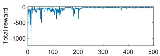
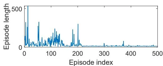
Figure 8.9: Sarsa with linear function approximation. Here, , , , , and .

Algorithm 8.2: Sarsa with function approximation
Initialization: Initial parameter . Initial policy . for all . .
Goal: Learn an optimal policy that can lead the agent to the target state from an initial state .
For each episode, do
Generate at following
If ( ) is not the target state, do
Collect the experience sample given : generate
by interacting with the environment; generate following .
Update q-value:
Update policy:
8.3.2 Q-learning with function approximation
Tabular Q-learning can also be extended to the case of function approximation. The update rule is
The above update rule is similar to (8.35) except that in (8.35) is replaced with .
Similar to the tabular case, (8.36) can be implemented in either an on-policy or off-policy fashion. An on-policy version is given in Algorithm 8.3. An example for demonstrating the on-policy version is shown in Figure 8.10. In this example, the task is to find a good policy that can lead the agent to the target state from the top-left state.
Algorithm 8.3: Q-learning with function approximation (on-policy version)
Initialization: Initial parameter . Initial policy . for all . .
Goal: Learn an optimal path that can lead the agent to the target state from an initial state .
For each episode, do
If ( ) is not the target state, do
Collect the experience sample given : generate following ; generate by interacting with the environment.
Update q-value:
Update policy:
As can be seen, Q-learning with linear function approximation can successfully learn an optimal policy. Here, linear Fourier basis functions of order five are used. The off-policy version will be demonstrated when we introduce deep Q-learning in Section 8.4.

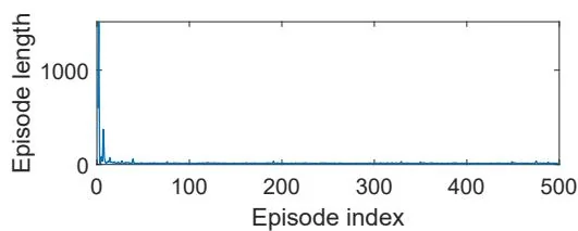
Figure 8.10: Q-learning with linear function approximation. Here, , , , , and .

One may notice in Algorithm 8.2 and Algorithm 8.3 that, although the values are represented as functions, the policy is still represented as a table. Thus, it still assumes finite numbers of states and actions. In Chapter 9, we will see that the policies can be represented as functions so that continuous state and action spaces can be handled.