3.7 Q&A

Q: What is the definition of optimal policies?

A: A policy is optimal if its corresponding state values are greater than or equal to any other policy.

It should be noted that this specific definition of optimality is valid only for tabular reinforcement learning algorithms. When the values or policies are approximated by functions, different metrics must be used to define optimal policies. This will become clearer in Chapters 8 and 9.

Q: Why is the Bellman optimality equation important?

A: It is important because it characterizes both optimal policies and optimal state values. Solving this equation yields an optimal policy and the corresponding optimal state value.

Q: Is the Bellman optimality equation a Bellman equation?

A: Yes. The Bellman optimality equation is a special Bellman equation whose corresponding policy is optimal.

Q: Is the solution of the Bellman optimality equation unique?

A: The Bellman optimality equation has two unknown variables. The first unknown variable is a value, and the second is a policy. The value solution, which is the optimal state value, is unique. The policy solution, which is an optimal policy, may not be unique.

Q: What is the key property of the Bellman optimality equation for analyzing its solution?

A: The key property is that the right-hand side of the Bellman optimality equation is a contraction mapping. As a result, we can apply the contraction mapping theorem to analyze its solution.

Q: Do optimal policies exist?

A: Yes. Optimal policies always exist according to the analysis of the BOE.

Q: Are optimal policies unique?

A: No. There may exist multiple or infinite optimal policies that have the same optimal state values.

Q: Are optimal policies stochastic or deterministic?

A: An optimal policy can be either deterministic or stochastic. A nice fact is that there always exist deterministic greedy optimal policies.

Q: How to obtain an optimal policy?

A: Solving the BOE using the iterative algorithm suggested by Theorem 3.3 yields an optimal policy. The detailed implementation of this iterative algorithm will be given in Chapter 4. Notably, all the reinforcement learning algorithms introduced in this book aim to obtain optimal policies under different settings.

Q: What is the general impact on the optimal policies if we reduce the value of the discount rate?

A: The optimal policy becomes more short-sighted when we reduce the discount rate. That is, the agent does not dare to take risks even though it may obtain greater cumulative rewards afterward.

Q: What happens if we set the discount rate to zero?

A: The resulting optimal policy would become extremely short-sighted. The agent would take the action with the greatest immediate reward, even though that action is not good in the long run.

Q: If we increase all the rewards by the same amount, will the optimal state value change? Will the optimal policy change?

A: Increasing all the rewards by the same amount is an affine transformation of the rewards, which would not affect the optimal policies. However, the optimal state value would increase, as shown in (3.8).

Q: If we hope that the optimal policy can avoid meaningless detours before reaching the target, should we add a negative reward to every step so that the agent reaches the target as quickly as possible?

A: First, introducing an additional negative reward to every step is an affine transformation of the rewards, which does not change the optimal policy. Second, the discount rate can automatically encourage the agent to reach the target as quickly as possible. This is because meaningless detours would increase the trajectory length and reduce the discounted return.

Chapter 4

Value Iteration and Policy Iteration

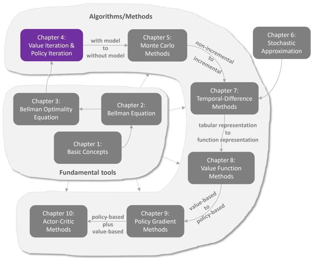
Figure 4.1: Where we are in this book.

With the preparation in the previous chapters, we are now ready to present the first algorithms that can find optimal policies. This chapter introduces three algorithms that are closely related to each other. The first is the value iteration algorithm, which is exactly the algorithm suggested by the contraction mapping theorem for solving the Bellman optimality equation as discussed in the last chapter. We focus more on the implementation details of this algorithm in the present chapter. The second is the policy iteration algorithm, whose idea is widely used in reinforcement learning algorithms. The third is the truncated policy iteration algorithm, which is a unified algorithm that includes the value iteration and policy iteration algorithms as special cases.

The algorithms introduced in this chapter are called dynamic programming algorithms [10, 11], which require the system model. These algorithms are important foundations of the model-free reinforcement learning algorithms introduced in the subsequent chapters. For example, the Monte Carlo algorithms introduced in Chapter 5 can be immediately obtained by extending the policy iteration algorithm introduced in this chapter.