7.7 Q&A

Q: What does the term "TD" in TD learning mean?

A: Every TD algorithm has a TD error, which represents the discrepancy between the new sample and the current estimate. Since this discrepancy is calculated between different time steps, it is called temporal-difference.

Q: What does the term "learning" in TD learning mean?

A: From a mathematical point of view, "learning" simply means "estimation". That is to estimate state/action values from some samples and then obtain policies based on the estimated values.

Q: While Sarsa can estimate the action values of a given policy, how can it be used to learn optimal policies?

A: To obtain an optimal policy, the value estimation process should interact with the policy improvement process. That is, after a value is updated, the corresponding policy should be updated. Then, the updated policy generates new samples that can be used to estimate values again. This is the idea of generalized policy iteration.

Q: Why does Sarsa update policies to be $\epsilon$ -greedy?

A: That is because the policy is also used to generate samples for value estimation. Hence, it should be exploratory to generate sufficient experience samples.

$\diamond$ Q: While Theorems 7.1 and 7.2 require that the learning rate $\alpha_{t}$ converges to zero gradually, why is it often set to be a small constant in practice?

A: The fundamental reason is that the policy to be evaluated keeps changing (or called nonstationary). In particular, a TD learning algorithm like Sarsa aims to estimate the action values of a given policy. If the policy is fixed, using a decaying learning rate is acceptable. However, in the optimal policy learning process, the policy that Sarsa aims to evaluate keeps changing after every iteration. We need a constant learning rate in this case; otherwise, a decaying learning rate may be too small to effectively evaluate policies. Although a drawback of constant learning rates is that the value estimate may fluctuate eventually, the fluctuation is negligible as long as the constant learning rate is sufficiently small.

Q: Should we learn the optimal policies for all states or a subset of the states?

A: It depends on the task. One may notice that some tasks considered in this chapter (e.g., Figure 7.2) do not require finding the optimal policies for all states. Instead, they only need to find an optimal path from a given starting state to the target state. Such tasks are not demanding in terms of data because the agent does not need to visit every state-action pair sufficiently many times. It, however, must be noted that the obtained path is not guaranteed to be optimal. That is because better paths may be missed if not all state-action pairs are well explored. Nevertheless, given sufficient data, we can still find a good or locally optimal path.

Q: Why is Q-learning off-policy while all the other TD algorithms in this chapter are on-policy?

A: The fundamental reason is that Q-learning aims to solve the Bellman optimality equation, whereas the other TD algorithms aim to solve the Bellman equation of a given policy. Details can be found in Section 7.4.2.

Q: Why does the off-policy version of Q-learning update policies to be greedy instead of $\epsilon$ -greedy?

A: That is because the target policy is not required to generate experience samples. Hence, it is not required to be exploratory.

Chapter 8

Value Function Methods

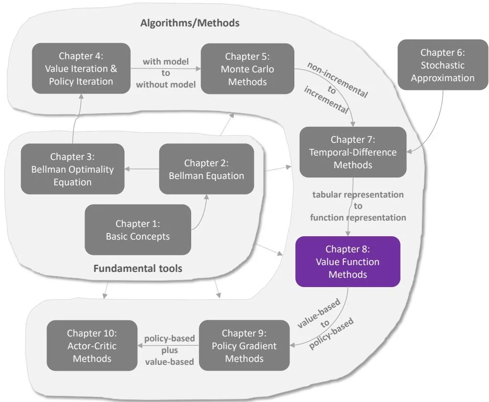
Figure 8.1: Where we are in this book.

In this chapter, we continue to study temporal-difference learning algorithms. However, a different method is used to represent state/action values. So far in this book, state/action values have been represented by tables. The tabular method is straightforward to understand, but it is inefficient for handling large state or action spaces. To solve this problem, this chapter introduces the value function method, which has become a standard way to represent values. It is also where artificial neural networks are incorporated into reinforcement learning as function approximators. The idea of value function can also be extended to policy function, as introduced in Chapter 9.

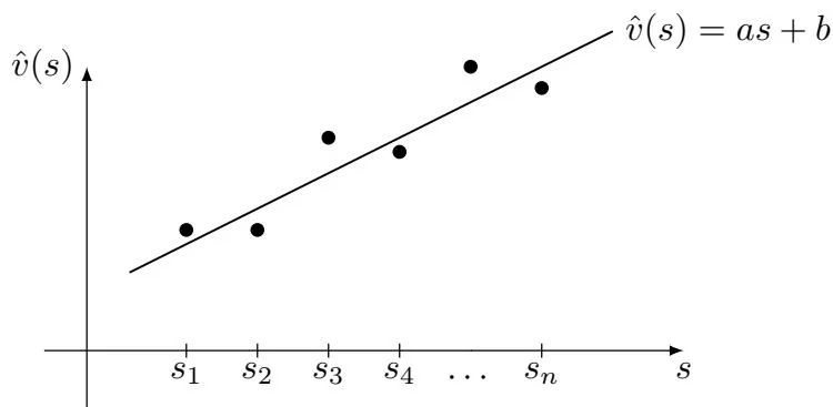
Figure 8.2: An illustration of the function approximation method. The x-axis and y-axis correspond to $s$ and $\hat{v}(s)$ , respectively.