1.6 Trajectories, returns, and episodes

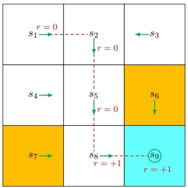
(a) Policy 1 and the trajectory

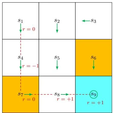
(b) Policy 2 and the trajectory
Figure 1.6: Trajectories obtained by following two policies. The trajectories are indicated by red dashed lines.

A trajectory is a state-action-reward chain. For example, given the policy shown in Figure 1.6(a), the agent can move along a trajectory as follows:

The return of this trajectory is defined as the sum of all the rewards collected along the trajectory:

Returns are also called total rewards or cumulative rewards.

Returns can be used to evaluate policies. For example, we can evaluate the two policies in Figure 1.6 by comparing their returns. In particular, starting from $s_1$ , the return obtained by the left policy is 1 as calculated above. For the right policy, starting from $s_1$ , the following trajectory is generated:

The corresponding return is

The returns in (1.1) and (1.2) indicate that the left policy is better than the right one since its return is greater. This mathematical conclusion is consistent with the intuition that the right policy is worse since it passes through a forbidden cell.

A return consists of an immediate reward and future rewards. Here, the immediate reward is the reward obtained after taking an action at the initial state; the future rewards refer to the rewards obtained after leaving the initial state. It is possible that the immediate reward is negative while the future reward is positive. Thus, which actions to take should be determined by the return (i.e., the total reward) rather than the immediate reward to avoid short-sighted decisions.

The return in (1.1) is defined for a finite-length trajectory. Return can also be defined for infinitely long trajectories. For example, the trajectory in Figure 1.6 stops after reaching $s_9$ . Since the policy is well defined for $s_9$ , the process does not have to stop after the agent reaches $s_9$ . We can design a policy so that the agent stays still after reaching $s_9$ . Then, the policy would generate the following infinitely long trajectory:

The direct sum of the rewards along this trajectory is

which unfortunately diverges. Therefore, we must introduce the discounted return concept for infinitely long trajectories. In particular, the discounted return is the sum of the discounted rewards:

where $\gamma \in (0,1)$ is called the discount rate. When $\gamma \in (0,1)$ , the value of (1.3) can be

calculated as

The introduction of the discount rate is useful for the following reasons. First, it removes the stop criterion and allows for infinitely long trajectories. Second, the discount rate can be used to adjust the emphasis placed on near- or far-future rewards. In particular, if $\gamma$ is close to 0, then the agent places more emphasis on rewards obtained in the near future. The resulting policy would be short-sighted. If $\gamma$ is close to 1, then the agent places more emphasis on the far future rewards. The resulting policy is far-sighted and dares to take risks of obtaining negative rewards in the near future. These points will be demonstrated in Section 3.5.

One important notion that was not explicitly mentioned in the above discussion is the episode. When interacting with the environment by following a policy, the agent may stop at some terminal states. The resulting trajectory is called an episode (or a trial). If the environment or policy is stochastic, we obtain different episodes when starting from the same state. However, if everything is deterministic, we always obtain the same episode when starting from the same state.

An episode is usually assumed to be a finite trajectory. Tasks with episodes are called episodic tasks. However, some tasks may have no terminal states, meaning that the process of interacting with the environment will never end. Such tasks are called continuing tasks. In fact, we can treat episodic and continuing tasks in a unified mathematical manner by converting episodic tasks to continuing ones. To do that, we need well define the process after the agent reaches the terminal state. Specifically, after reaching the terminal state in an episodic task, the agent can continue taking actions in the following two ways.

$\diamond$ First, if we treat the terminal state as a special state, we can specifically design its action space or state transition so that the agent stays in this state forever. Such states are called absorbing states, meaning that the agent never leaves a state once reached. For example, for the target state $s_9$ , we can specify $\mathcal{A}(s_9) = \{a_5\}$ or set $\mathcal{A}(s_9) = \{a_1, \ldots, a_5\}$ with $p(s_9 | s_9, a_i) = 1$ for all $i = 1, \ldots, 5$ .
$\diamond$ Second, if we treat the terminal state as a normal state, we can simply set its action space to the same as the other states, and the agent may leave the state and come back again. Since a positive reward of $r = 1$ can be obtained every time $s_9$ is reached, the agent will eventually learn to stay at $s_9$ forever to collect more rewards. Notably, when an episode is infinitely long and the reward received for staying at $s_9$ is positive, a discount rate must be used to calculate the discounted return to avoid divergence.

In this book, we consider the second scenario where the target state is treated as a normal state whose action space is $\mathcal{A}(s_9) = \{a_1,\ldots ,a_5\}$ .