This section presents another important algorithm: policy iteration. Unlike value iteration, policy iteration is not for directly solving the Bellman optimality equation. However, it has an intimate relationship with value iteration, as shown later. Moreover, the idea of policy iteration is very important since it is widely utilized in reinforcement learning algorithms.
4.2.1 Algorithm analysis
Policy iteration is an iterative algorithm. Each iteration has two steps.
The first is a policy evaluation step. As its name suggests, this step evaluates a given policy by calculating the corresponding state value. That is to solve the following Bellman equation:
vπk=rπk+γPπkvπk,(4.3)
where πk is the policy obtained in the last iteration and vπk is the state value to be calculated. The values of rπk and Pπk can be obtained from the system model.
⋄ The second is a policy improvement step. As its name suggests, this step is used to improve the policy. In particular, once vπk has been calculated in the first step, a new policy πk+1 can be obtained as
πk+1=argπmax(rπ+γPπvπk).
Three questions naturally follow the above description of the algorithm.
In the policy evaluation step, how to solve the state value vπk ? In the policy improvement step, why is the new policy πk+1 better than πk ? ⋄ Why can this algorithm finally converge to an optimal policy?
We next answer these questions one by one.
In the policy evaluation step, how to calculate vπk ?
We introduced two methods in Chapter 2 for solving the Bellman equation in (4.3). We next revisit the two methods briefly. The first method is a closed-form solution:
4.2. Policy iteration
vπk=(I−γPπk)−1rπk . This closed-form solution is useful for theoretical analysis purposes, but it is inefficient to implement since it requires other numerical algorithms to compute the matrix inverse. The second method is an iterative algorithm that can be easily implemented:
vπk(j+1)=rπk+γPπkvπk(j),j=0,1,2,…(4.4)
where vπk(j) denotes the j th estimate of vπk . Starting from any initial guess vπk(0) , it is ensured that vπk(j)→vπk as j→∞ . Details can be found in Section 2.7.
Interestingly, policy iteration is an iterative algorithm with another iterative algorithm (4.4) embedded in the policy evaluation step. In theory, this embedded iterative algorithm requires an infinite number of steps (that is, j→∞ ) to converge to the true state value vπk . This is, however, impossible to realize. In practice, the iterative process terminates when a certain criterion is satisfied. For example, the termination criterion can be that ∥vπk(j+1)−vπk(j)∥ is less than a prespecified threshold or that j exceeds a prespecified value. If we do not run an infinite number of iterations, we can only obtain an imprecise value of vπk , which will be used in the subsequent policy improvement step. Would this cause problems? The answer is no. The reason will become clear when we introduce the truncated policy iteration algorithm later in Section 4.3.
In the policy improvement step, why is πk+1 better than πk ?
The policy improvement step can improve the given policy, as shown below.
Lemma 4.1 (Policy improvement). If πk+1=argmaxπ(rπ+γPπvπk) , then vπk+1≥vπk
Here, vπk+1≥vπk means that vπk+1(s)≥vπk(s) for all s . The proof of this lemma is given in Box 4.1.
Box 4.1: Proof of Lemma 4.1
Since vπk+1 and vπk are state values, they satisfy the Bellman equations:
vπk+1=rπk+1+γPπk+1vπk+1,
vπk=rπk+γPπkvπk.
Since πk+1=argmaxπ(rπ+γPπvπk) , we know that
The limit is due to the facts that γn→0 as n→∞ and Pπk+1n is a nonnegative stochastic matrix for any n . Here, a stochastic matrix refers to a nonnegative matrix whose row sums are equal to one for all rows.
Why can the policy iteration algorithm eventually find an optimal policy?
The policy iteration algorithm generates two sequences. The first is a sequence of policies: {π0,π1,…,πk,…} . The second is a sequence of state values: {vπ0,vπ1,…,vπk,…} . Suppose that v∗ is the optimal state value. Then, vπk≤v∗ for all k . Since the policies are continuously improved according to Lemma 4.1, we know that
vπ0≤vπ1≤vπ2≤⋯≤vπk≤⋯≤v∗.
Since vπk is nondecreasing and always bounded from above by v∗ , it follows from the monotone convergence theorem [12] (Appendix C) that vπk converges to a constant value, denoted as v∞ , when k→∞ . The following analysis shows that v∞=v∗ .
Theorem 4.1 (Convergence of policy iteration). The state value sequence {vπk}k=0∞ generated by the policy iteration algorithm converges to the optimal state value v∗ . As a result, the policy sequence {πk}k=0∞ converges to an optimal policy.
The proof of this theorem is given in Box 4.2. The proof not only shows the convergence of the policy iteration algorithm but also reveals the relationship between the policy iteration and value iteration algorithms. Loosely speaking, if both algorithms start from the same initial guess, policy iteration will converge faster than value iteration due to the additional iterations embedded in the policy evaluation step. This point will become clearer when we introduce the truncated policy iteration algorithm in Section 4.3.
Box 4.2: Proof of Theorem 4.1
The idea of the proof is to show that the policy iteration algorithm converges faster than the value iteration algorithm.
In particular, to prove the convergence of {vπk}k=0∞ , we introduce another sequence {vk}k=0∞ generated by
vk+1=f(vk)=πmax(rπ+γPπvk).
This iterative algorithm is exactly the value iteration algorithm. We already know that vk converges to v∗ when given any initial value v0 .
For k=0 , we can always find a v0 such that vπ0≥v0 for any π0 .
We next show that vk≤vπk≤v∗ for all k by induction.
For k≥0 , suppose that vπk≥vk .
For k+1 , we have
vπk+1−vk+1=(rπk+1+γPπk+1vπk+1)−maxπ(rπ+γPπvk)≥(rπk+1+γPπk+1vπk)−maxπ(rπ+γPπvk)(becausevπk+1≥vπkbyLemma4.1andPπk+1≥0)=(rπk+1+γPπk+1vπk)−(rπk′+γPπk′vk)(s u p p o s eπk′=argmaxπ(rπ+γPπvk))≥(rπk′+γPπk′vπk)−(rπk′+γPπk′vk)(b e c a u s eπk+1=argmaxπ(rπ+γPπvπk))=γPπk′(vπk−vk).
Since vπk−vk≥0 and Pπk′ is nonnegative, we have Pπk′(vπk−vk)≥0 and hence vπk+1−vk+1≥0 .
Therefore, we can show by induction that vk≤vπk≤v∗ for any k≥0 . Since vk converges to v∗ , vπk also converges to v∗ .
4.2.2 Elementwise form and implementation
To implement the policy iteration algorithm, we need to study its elementwise form.
⋄ First, the policy evaluation step solves vπk from vπk=rπk+γPπkvπk by using the
Algorithm 4.2: Policy iteration algorithm
Initialization: The system model, p(r∣s,a) and p(s′∣s,a) for all (s,a) , is known. Initial guess π0 .
Goal: Search for the optimal state value and an optimal policy.
While vπk has not converged, for the k th iteration, do
Policy evaluation:
Initialization: an arbitrary initial guess vπk(0)
While vπk(j) has not converged, for the j th iteration, do
where qπk(s,a) is the action value under policy πk . Let ak∗(s)=argmaxaqπk(s,a) . Then, the greedy optimal policy is
πk+1(a∣s)={1,0,a=ak∗(s),a=ak∗(s).
The implementation details are summarized in Algorithm 4.2.
4.2.3 Illustrative examples
A simple example
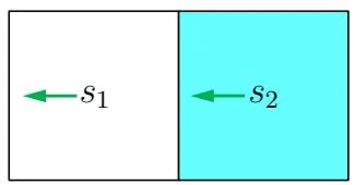
Consider a simple example shown in Figure 4.3. There are two states with three possible actions: A={aℓ,a0,ar} . The three actions represent moving leftward, staying unchanged, and moving rightward. The reward settings are rboundary=−1 and rtarget=1 . The discount rate is γ=0.9 .
(a)
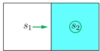
(b) Figure 4.3: An example for illustrating the implementation of the policy iteration algorithm.
We next present the implementation of the policy iteration algorithm in a step-by-step manner. When k=0 , we start with the initial policy shown in Figure 4.3(a). This policy is not good because it does not move toward the target area. We next show how to apply the policy iteration algorithm to obtain an optimal policy.
First, in the policy evaluation step, we need to solve the Bellman equation:
vπ0(s1)=−1+γvπ0(s1),
vπ0(s2)=0+γvπ0(s1).
Since the equation is simple, it can be manually solved that
vπ0(s1)=−10,vπ0(s2)=−9.
In practice, the equation can be solved by the iterative algorithm in (4.4). For example, select the initial state values as vπ0(0)(s1)=vπ0(0)(s2)=0 . It follows from (4.4) that
With more iterations, we can see the trend: vπ0(j)(s1)→vπ0(s1)=−10 and vπ0(j)(s2)→vπ0(s2)=−9 as j increases.
⋄ Second, in the policy improvement step, the key is to calculate qπ0(s,a) for each state-action pair. The following q-table can be used to demonstrate such a process:
Substituting vπ0(s1)=−10,vπ0(s2)=−9 obtained in the previous policy evaluation step into Table 4.4 yields Table 4.5.
Table 4.4: The expression of qπk(s,a) for the example in Figure 4.3.
Table 4.5: The value of qπk(s,a) when k=0 .
By seeking the greatest value of qπ0 , the improved policy π1 can be obtained as
π1(ar∣s1)=1,π1(a0∣s2)=1.
This policy is illustrated in Figure 4.3(b). It is clear that this policy is optimal.
The above process shows that a single iteration is sufficient for finding the optimal policy in this simple example. More iterations are required for more complex examples.
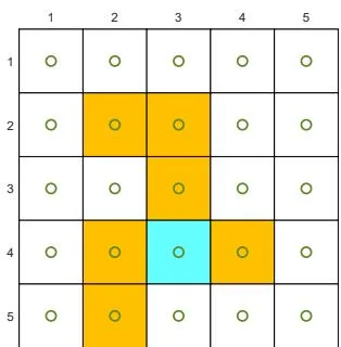
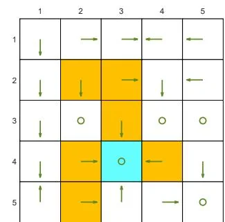
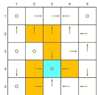
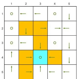
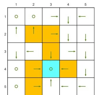
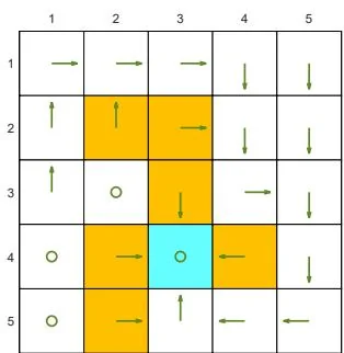
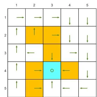
A more complicated example
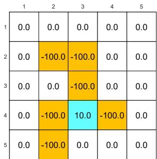
We next demonstrate the policy iteration algorithm using a more complicated example shown in Figure 4.4. The reward settings are rboundary=−1 , rforbidden=−10 , and rtarget=1 . The discount rate is γ=0.9 . The policy iteration algorithm can converge to the optimal policy (Figure 4.4(h)) when starting from a random initial policy (Figure 4.4(a)).
Two interesting phenomena are observed during the iteration process.
⋄ First, if we observe how the policy evolves, an interesting pattern is that the states that are close to the target area find the optimal policies earlier than those far away. Only if the close states can find trajectories to the target first, can the farther states find trajectories passing through the close states to reach the target. ⋄ Second, the spatial distribution of the state values exhibits an interesting pattern: the states that are located closer to the target have greater state values. The reason for this pattern is that an agent starting from a farther state must travel for many steps to obtain a positive reward. Such rewards would be severely discounted and hence relatively small.
(a) π0 and vπ0
(b) π1 and vπ1
(c) π2 and vπ2
(d) π3 and vπ3
(e) π4 and vπ4
(f) π5 and vπ5
(g) π9 and vπ9
Figure 4.4: The evolution processes of the policies generated by the policy iteration algorithm.