2.2 Motivating example 2: How to calculate returns?
While we have demonstrated the importance of returns, a question that immediately follows is how to calculate the returns when following a given policy.
There are two ways to calculate returns.
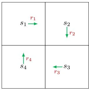
The first is simply by definition: a return equals the discounted sum of all the rewards collected along a trajectory. Consider the example in Figure 2.3. Let vi denote the return obtained by starting from si for i=1,2,3,4 . Then, the returns obtained when
Figure 2.3: An example for demonstrating how to calculate returns. There are no target or forbidden cells in this example.
starting from the four states in Figure 2.3 can be calculated as
v1=r1+γr2+γ2r3+…,
v2=r2+γr3+γ2r4+…,(2.2)
v3=r3+γr4+γ2r1+…,
v4=r4+γr1+γ2r2+….
The second way, which is more important, is based on the idea of bootstrapping. By observing the expressions of the returns in (2.2), we can rewrite them as
v1=r1+γ(r2+γr3+…)=r1+γv2,
v2=r2+γ(r3+γr4+…)=r2+γv3,(2.3)
v3=r3+γ(r4+γr1+…)=r3+γv4,
v4=r4+γ(r1+γr2+…)=r4+γv1.
The above equations indicate an interesting phenomenon that the values of the returns rely on each other. More specifically, v1 relies on v2 , v2 relies on v3 , v3 relies on v4 , and v4 relies on v1 . This reflects the idea of bootstrapping, which is to obtain the values of some quantities from themselves.
At first glance, bootstrapping is an endless loop because the calculation of an unknown value relies on another unknown value. In fact, bootstrapping is easier to understand if we view it from a mathematical perspective. In particular, the equations in (2.3) can be reformed into a linear matrix-vector equation:
Thus, the value of v can be calculated easily as v=(I−γP)−1r , where I is the identity matrix with appropriate dimensions. One may ask whether I−γP is always invertible. The answer is yes and explained in Section 2.7.1.
In fact, (2.3) is the Bellman equation for this simple example. Although it is simple, (2.3) demonstrates the core idea of the Bellman equation: the return obtained by starting from one state depends on those obtained when starting from other states. The idea of bootstrapping and the Bellman equation for general scenarios will be formalized in the following sections.