5.7 Q&A

Q: What is Monte Carlo estimation?

A: Monte Carlo estimation refers to a broad class of techniques that use stochastic samples to solve approximation problems.

Q: What is the mean estimation problem?

A: The mean estimation problem refers to calculating the expected value of a random variable based on stochastic samples.

Q: How to solve the mean estimation problem?

A: There are two approaches: model-based and model-free. In particular, if the probability distribution of a random variable is known, the expected value can be calculated

based on its definition. If the probability distribution is unknown, we can use Monte Carlo estimation to approximate the expected value. Such an approximation is accurate when the number of samples is large.

Q: Why is the mean estimation problem important for reinforcement learning?

A: Both state and action values are defined as expected values of returns. Hence, estimating state or action values is essentially a mean estimation problem.

Q: What is the core idea of model-free MC-based reinforcement learning?

A: The core idea is to convert the policy iteration algorithm to a model-free one. In particular, while the policy iteration algorithm aims to calculate values based on the system model, MC-based reinforcement learning replaces the model-based policy evaluation step in the policy iteration algorithm with a model-free MC-based policy evaluation step.

Q: What are initial-visit, first-visit, and every-visit strategies?

A: They are different strategies for utilizing the samples in an episode. An episode may visit many state-action pairs. The initial-visit strategy uses the entire episode to estimate the action value of the initial state-action pair. The every-visit and first-visit strategies can better utilize the given samples. If the rest of the episode is used to estimate the action value of a state-action pair every time it is visited, such a strategy is called every-visit. If we only count the first time a state-action pair is visited in the episode, such a strategy is called first-visit.

Q: What is exploring starts? Why is it important?

A: Exploring starts requires an infinite number of (or sufficiently many) episodes to be generated when starting from every state-action pair. In theory, the exploring starts condition is necessary to find optimal policies. That is, only if every action value is well explored, can we accurately evaluate all the actions and then correctly select the optimal ones.

Q: What is the idea used to avoid exploring starts?

A: The fundamental idea is to make policies soft. Soft policies are stochastic, enabling an episode to visit many state-action pairs. In this way, we do not need a large number of episodes starting from every state-action pair.

Q: Can an $\epsilon$ -greedy policy be optimal?

A: The answer is both yes and no. By yes, we mean that, if given sufficient samples, the MC $\epsilon$ -Greedy algorithm can converge to an optimal $\epsilon$ -greedy policy. By no, we mean that the converged policy is merely optimal among all $\epsilon$ -greedy policies (with the same value of $\epsilon$ ).

Q: Is it possible to use one episode to visit all state-action pairs?

A: Yes, it is possible. If the policy is soft (e.g., $\epsilon$ -greedy) and the episode is sufficiently long.

Q: What is the relationship between MC Basic, MC Exploring Starts, and MC €-Greedy?

A: MC Basic is the simplest MC-based reinforcement learning algorithm. It is important because it reveals the fundamental idea of model-free MC-based reinforcement learning. MC Exploring Starts is a variant of MC Basic that adjusts the sample usage strategy. Furthermore, MC $\epsilon$ -Greedy is a variant of MC Exploring Starts that removes the exploring starts requirement. Therefore, while the basic idea is simple, complication appears when we want to achieve better performance. It is important to split the core idea from the complications that may be distracting for beginners.

Chapter 6

Stochastic Approximation

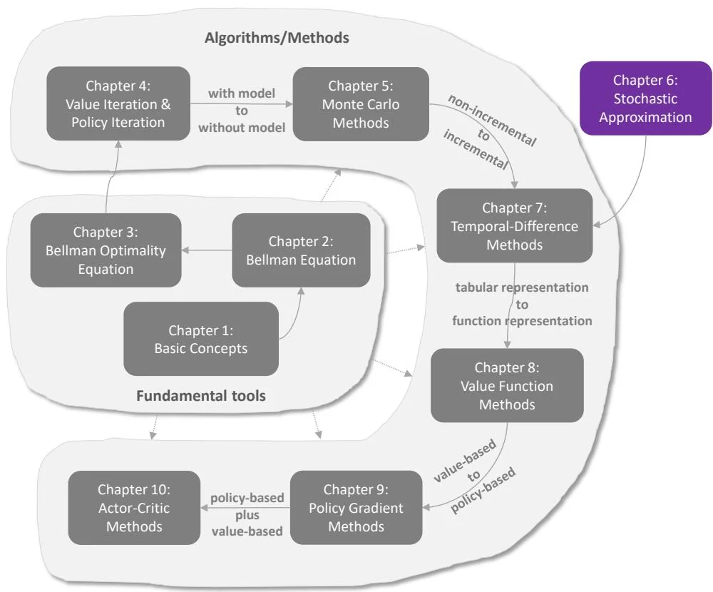
Figure 6.1: Where we are in this book.

Chapter 5 introduced the first class of model-free reinforcement learning algorithms based on Monte Carlo estimation. In the next chapter (Chapter 7), we will introduce another class of model-free reinforcement learning algorithms: temporal-difference learning. However, before proceeding to the next chapter, we need to press the pause button to better prepare ourselves. This is because temporal-difference algorithms are very different from the algorithms that we have studied so far. Many readers who see the temporal-difference algorithms for the first time often wonder how these algorithms were designed in the first place and why they can work effectively. In fact, there is a knowledge gap between the previous and subsequent chapters: the algorithms we have studied so far are

non-incremental, but the algorithms that we will study in the subsequent chapters are incremental.

We use the present chapter to fill this knowledge gap by introducing the basics of stochastic approximation. Although this chapter does not introduce any specific reinforcement learning algorithms, it lays the necessary foundations for studying subsequent chapters. We will see in Chapter 7 that the temporal-difference algorithms can be viewed as special stochastic approximation algorithms. The well-known stochastic gradient descent algorithms widely used in machine learning are also introduced in the present chapter.