14.1_Introduction
14.1 Introduction
Given bodies with positions and velocities for , the force vector on body caused by body is given by
where and are the masses of bodies and , respectively; is the difference vector from body to body ; and is the gravitational constant. Due to divide overflow, this express diverges for with small magnitude; to compensate, it is common practice to apply a softening factor that models the interaction between two Plummer masses—masses that behave as if they were spherical galaxies. For a softening factor , the resulting expression is
The total force on body , due to its interactions with the other bodies, is obtained by summing all interactions.
To update the position and velocity of each body, the force (acceleration) applied for body is , so the term can be removed from the numerator, as follows.
Like Nyland et al., we use a leapfrog Verlet algorithm to apply a timestep to the simulation. The values of the positions and velocities are offset by half a timestep from one another, a characteristic that is not obvious from the code
because in our sample, the positions and velocities are initially assigned random values. Our leapfrog Verlet integration updates the velocity, then the position.
This method is just one of many different integration algorithms that can be used to update the simulation, but an extensive discussion is outside the scope of this book.
Since the integration has a runtime of and computing the forces has a runtime of , the biggest performance benefits from porting to CUDA stem from optimizing the force computation. Optimizing this portion of the calculation is the primary focus of this chapter.
14.1.1 A MATRIX OF FORCES
A naive implementation of the N-Body algorithm consists of a doubly nested loop that, for each body, computes the sum of the forces exerted on that body by every other body. The body-body forces can be thought of as an matrix, where the sum of each row is the total gravitational force exerted on body .
The diagonals of this "matrix" are zeroes corresponding to each body's influence on itself, which can be ignored.
Because each element in the matrix may be computed independently, there is a tremendous amount of potential parallelism. The sum of each row is a reduction that may be computed by a single thread or by combining results from multiple threads as described in Chapter 12.
Figure 14.1 shows an 8-body "matrix" being processed. The rows correspond to the sums that are the output of the computation. When using CUDA, N-Body implementations typically have one thread compute the sum for each row.
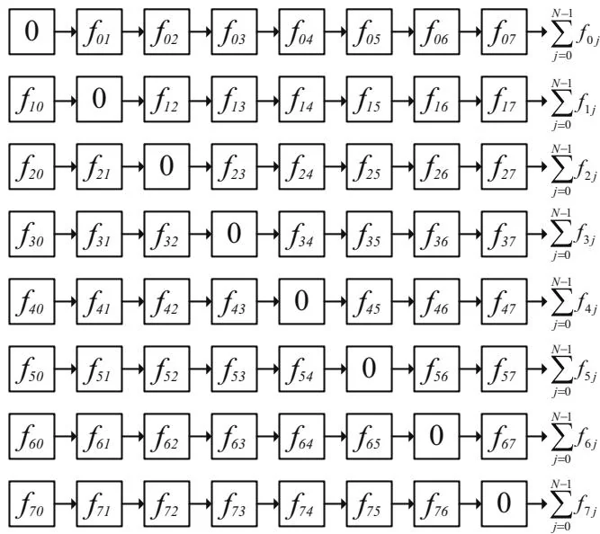
Figure 14.1 "Matrix" of forces (8 bodies).
Since every element in the "matrix" is independent, they also may be computed in parallel within a given row: Compute the sum of every fourth element, for example, and then add the four partial sums to compute the final output. Harris et al. describe using this method for small where there are not enough threads to cover the latencies in the GPU: Launch more threads, compute partial sums in each thread, and accumulate the final sums with reductions in shared memory. Harris et al. reported a benefit for .
For physical forces that are symmetric (i.e., the force exerted on body by body is equal in magnitude but has the opposite sign of the force exerted by body on ), such as gravitation, the transpose "elements" of the matrix have the opposite sign.
In this case, the "matrix" takes the form shown in Figure 14.2. When exploiting the symmetry, an implementation need only compute the upper right triangle of the "matrix," performing about half as many body-body computations.
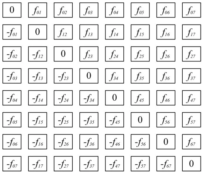
Figure 14.2 Matrix with symmetric forces.
The problem is that unlike the brute force method outlined in Figure 14.1, when exploiting symmetric forces, different threads may have contributions to add to a given output sum. Partial sums must be accumulated and either written to temporary locations for eventual reduction or the system must protect the final sums with mutual exclusion (by using atomics or thread synchronization). Since the body-body computation is about 20 FLOPS (for single precision) or 30 FLOPS (for double precision), subtracting from a sum would seem like a decisive performance win.
Unfortunately, the overhead often overwhelms the benefit of performing half as many body-body computations. For example, a completely naive implementation that does two (2) floating-point atomic adds per body-body computation is prohibitively slower than the brute force method.
Figure 14.3 shows a compromise between the two extremes: By tiling the computation, only the upper right diagonal of tiles needs to be computed. For a tile size of , this method performs body-body computations each on nondiagonal tiles, plus body-body computations each on
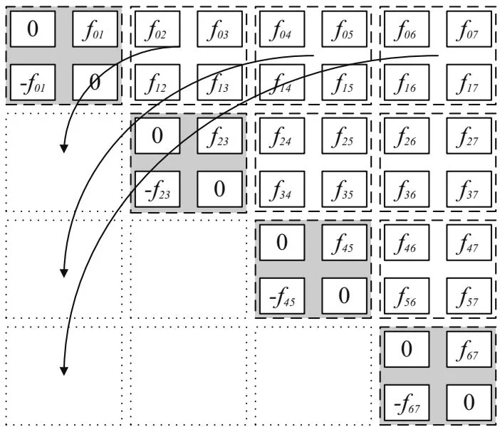
Figure 14.3 Tiled N-Body .
diagonal tiles. For large , the savings in body-body computations are about the same,[4] but because the tiles can locally accumulate partial sums to contribute to the final answer, the synchronization overhead is reduced. Figure 14.3 shows a tile size with , but a tile size corresponding to the warp size ( ) is more practical.
Figure 14.4 shows how the partial sums for a given tile are computed. The partial sums for the rows and columns are computed—adding and subtracting, respectively—in order to arrive at partial sums that must be added to the corresponding output sums.
The popular AMBER application for molecular modeling exploits symmetry of forces, performing the work on tiles tuned to the warp size of , but in extensive testing, the approach has not proven fruitful for the more lightweight computation described here.
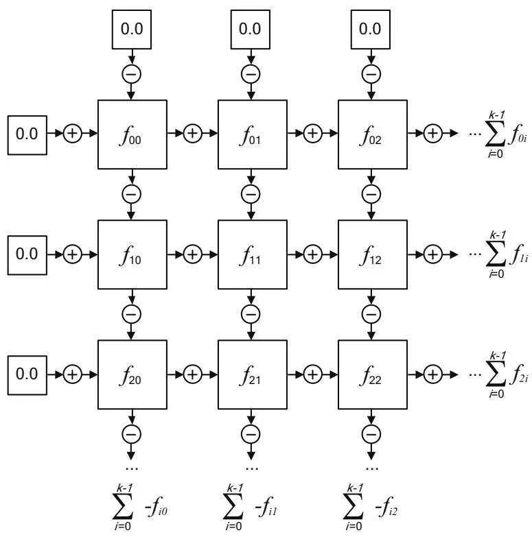
Figure 14.4 N-Body tile.