4.1 Value iteration

This section introduces the value iteration algorithm. It is exactly the algorithm suggested by the contraction mapping theorem for solving the Bellman optimality equation, as introduced in the last chapter (Theorem 3.3). In particular, the algorithm is

It is guaranteed by Theorem 3.3 that $v_{k}$ and $\pi_{k}$ converge to the optimal state value and an optimal policy as $k\to \infty$ , respectively.

This algorithm is iterative and has two steps in every iteration.

The first step in every iteration is a policy update step. Mathematically, it aims to find a policy that can solve the following optimization problem:

where $v_{k}$ is obtained in the previous iteration.

The second step is called a value update step. Mathematically, it calculates a new value $v_{k+1}$ by

where $v_{k + 1}$ will be used in the next iteration.

The value iteration algorithm introduced above is in a matrix-vector form. To implement this algorithm, we need to further examine its elementwise form. While the matrix-vector form is useful for understanding the core idea of the algorithm, the elementwise form is necessary for explaining the implementation details.

4.1.1 Elementwise form and implementation

Consider the time step $k$ and a state $s$ .

$\diamond$ First, the elementwise form of the policy update step $\pi_{k + 1} = \arg \max_{\pi}(r_{\pi} + \gamma P_{\pi}v_{k})$ is

We showed in Section 3.3.1 that the optimal policy that can solve the above optimization problem is

where $a_{k}^{*}(s) = \arg \max_{a} q_{k}(s, a)$ . If $a_{k}^{*}(s) = \arg \max_{a} q_{k}(s, a)$ has multiple solutions, we can select any of them without affecting the convergence of the algorithm. Since the new policy $\pi_{k+1}$ selects the action with the greatest $q_{k}(s, a)$ , such a policy is called greedy.

Second, the elementwise form of the value update step $v_{k + 1} = r_{\pi_{k + 1}} + \gamma P_{\pi_{k + 1}}v_k$ is

Substituting (4.2) into the above equation gives

In summary, the above steps can be illustrated as

The implementation details are summarized in Algorithm 4.1.

One problem that may be confusing is whether $v_{k}$ in (4.1) is a state value. The answer is no. Although $v_{k}$ eventually converges to the optimal state value, it is not ensured to satisfy the Bellman equation of any policy. For example, it does not satisfy $v_{k} = r_{\pi_{k + 1}} + \gamma P_{\pi_{k + 1}}v_{k}$ or $v_{k} = r_{\pi_{k}} + \gamma P_{\pi_{k}}v_{k}$ in general. It is merely an intermediate value generated by the algorithm. In addition, since $v_{k}$ is not a state value, $q_{k}$ is not an action value.

4.1.2 Illustrative examples

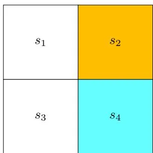
We next present an example to illustrate the step-by-step implementation of the value iteration algorithm. This example is a two-by-two grid with one forbidden area (Fig-

Algorithm 4.1: Value iteration algorithm

Initialization: The probability models $p(r|s,a)$ and $p(s'|s,a)$ for all $(s,a)$ are known. Initial guess $v_0$ .

Goal: Search for the optimal state value and an optimal policy for solving the Bellman optimality equation.

While $v_{k}$ has not converged in the sense that $\| v_{k} - v_{k-1} \|$ is greater than a predefined small threshold, for the $k$ th iteration, do

For every state $s \in S$ , do

For every action $a \in \mathcal{A}(s)$ , do

Maximum action value: $a_k^*(s) = \arg \max_a q_k(s, a)$

Policy update: $\pi_{k + 1}(a|s) = 1$ if $a = a_k^*$ , and $\pi_{k + 1}(a|s) = 0$ otherwise.

Value update: $v_{k+1}(s) = \max_a q_k(s, a)$

Table 4.1: The expression of $q(s, a)$ for the example as shown in Figure 4.2.

ure 4.2). The target area is $s_4$ . The reward settings are $r_{\mathrm{boundary}} = r_{\mathrm{forbidden}} = -1$ and $r_{\mathrm{target}} = 1$ . The discount rate is $\gamma = 0.9$ .

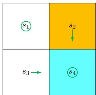
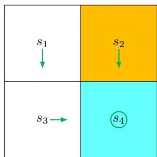
Figure 4.2: An example for demonstrating the implementation of the value iteration algorithm.

The expression of the q-value for each state-action pair is shown in Table 4.1.

Without loss of generality, select the initial values as $v_{0}(s_{1}) = v_{0}(s_{2}) = v_{0}(s_{3}) = v_{0}(s_{4}) = 0$ .

q-value calculation: Substituting $v_{0}(s_{i})$ into Table 4.1 gives the q-values shown in Table 4.2.

Table 4.2: The value of $q(s,a)$ at $k = 0$ .

Table 4.3: The value of $q\left( {s,a}\right)$ at $k = 1$ .

Policy update: $\pi_1$ is obtained by selecting the actions with the greatest q-values for every state:

This policy is visualized in Figure 4.2 (the middle subfigure). It is clear that this policy is not optimal because it selects to stay still at $s_1$ . Notably, the q-values for $(s_1, a_5)$ and $(s_1, a_3)$ are actually the same, and we can randomly select either action.

Value update: $v_{1}$ is obtained by updating the v-value to the greatest q-value for each state:

$k = 1$

q-value calculation: Substituting $v_{1}(s_{i})$ into Table 4.1 yields the q-values shown in Table 4.3.

Policy update: $\pi_{2}$ is obtained by selecting the greatest q-values:

This policy is visualized in Figure 4.2 (the right subfigure).

Value update: $v_{2}$ is obtained by updating the v-value to the greatest q-value for each state:

$k = 2,3,4,\ldots$

It is notable that policy $\pi_2$ , as illustrated in Figure 4.2, is already optimal. Therefore, we

4.2. Policy iteration

only need to run two iterations to obtain an optimal policy in this simple example. For more complex examples, we need to run more iterations until the value of $v_{k}$ converges (e.g., until $\| v_{k + 1} - v_k\|$ is smaller than a pre-specified threshold).