6.2 Robbins-Monro algorithm

Stochastic approximation refers to a broad class of stochastic iterative algorithms for solving root-finding or optimization problems [24]. Compared to many other root-finding

algorithms such as gradient-based ones, stochastic approximation is powerful in the sense that it does not require the expression of the objective function or its derivative.

The Robbins-Monro (RM) algorithm is a pioneering work in the field of stochastic approximation [24-27]. The famous stochastic gradient descent algorithm is a special form of the RM algorithm, as shown in Section 6.4. We next introduce the details of the RM algorithm.

Suppose that we would like to find the root of the equation

where $w \in \mathbb{R}$ is the unknown variable and $g: \mathbb{R} \to \mathbb{R}$ is a function. Many problems can be formulated as root-finding problems. For example, if $J(w)$ is an objective function to be optimized, this optimization problem can be converted to solving $g(w) \doteq \nabla_w J(w) = 0$ . In addition, an equation such as $g(w) = c$ , where $c$ is a constant, can also be converted to the above equation by rewriting $g(w) - c$ as a new function.

If the expression of $g$ or its derivative is known, there are many numerical algorithms that can be used. However, the problem we are facing is that the expression of the function $g$ is unknown. For example, the function may be represented by an artificial neural network whose structure and parameters are unknown. Moreover, we can only obtain a noisy observation of $g(w)$ :

where $\eta \in \mathbb{R}$ is the observation error, which may or may not be Gaussian. In summary, it is a black-box system where only the input $w$ and the noisy output $\tilde{g}(w, \eta)$ are known (see Figure 6.2). Our aim is to solve $g(w) = 0$ using $w$ and $\tilde{g}$ .

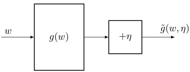
Figure 6.2: An illustration of the problem of solving $g(w) = 0$ from $w$ and $\tilde{g}$ .

The RM algorithm that can solve $g(w) = 0$ is

where $w_{k}$ is the $k$ th estimate of the root, $\tilde{g}(w_{k}, \eta_{k})$ is the $k$ th noisy observation, and $a_{k}$ is a positive coefficient. As can be seen, the RM algorithm does not require any information about the function. It only requires the input and output.

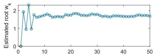
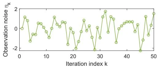
Figure 6.3: An illustrative example of the RM algorithm.

To illustrate the RM algorithm, consider an example in which $g(w) = w^3 - 5$ . The true root is $5^{1/3} \approx 1.71$ . Now, suppose that we can only observe the input $w$ and the output $\tilde{g}(w) = g(w) + \eta$ , where $\eta$ is i.i.d. and obeys a standard normal distribution with a zero mean and a standard deviation of 1. The initial guess is $w_1 = 0$ , and the coefficient is $a_k = 1/k$ . The evolution process of $w_k$ is shown in Figure 6.3. Even though the observation is corrupted by noise $\eta_k$ , the estimate $w_k$ can still converge to the true root. Note that the initial guess $w_1$ must be properly selected to ensure convergence for the specific function of $g(w) = w^3 - 5$ . In the following subsection, we present the conditions under which the RM algorithm converges for any initial guesses.

6.2.1 Convergence properties

Why can the RM algorithm in (6.5) find the root of $g(w) = 0$ ? We next illustrate the idea with an example and then provide a rigorous convergence analysis.

Consider the example shown in Figure 6.4. In this example, $g(w) = \tanh (w - 1)$ . The true root of $g(w) = 0$ is $w^{*} = 1$ . We apply the RM algorithm with $w_{1} = 3$ and $a_{k} = 1 / k$ . To better illustrate the reason for convergence, we simply set $\eta_k\equiv 0$ , and consequently, $\tilde{g} (w_k,\eta_k) = g(w_k)$ . The RM algorithm in this case is $w_{k + 1} = w_{k} - a_{k}g(w_{k})$ . The resulting $\{w_k\}$ generated by the RM algorithm is shown in Figure 6.4. It can be seen that $w_{k}$ converges to the true root $w^{*} = 1$ .

This simple example can illustrate why the RM algorithm converges.

$\diamond$ When $w_{k} > w^{*}$ , we have $g(w_{k}) > 0$ . Then, $w_{k + 1} = w_{k} - a_{k}g(w_{k}) < w_{k}$ . If $a_{k}g(w_{k})$ is sufficiently small, we have $w^{*} < w_{k + 1} < w_{k}$ . As a result, $w_{k + 1}$ is closer to $w^{*}$ than $w_{k}$ .
$\diamond$ When $w_{k} < w^{*}$ , we have $g(w_{k}) < 0$ . Then, $w_{k + 1} = w_{k} - a_{k}g(w_{k}) > w_{k}$ . If $|a_{k}g(w_{k})|$ is sufficiently small, we have $w^{*} > w_{k + 1} > w_{k}$ . As a result, $w_{k + 1}$ is closer to $w^{*}$ than $w_{k}$ .

In either case, $w_{k+1}$ is closer to $w^*$ than $w_k$ . Therefore, it is intuitive that $w_k$ converges to $w^*$ .

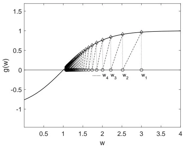
Figure 6.4: An example for illustrating the convergence of the RM algorithm.

The above example is simple since the observation error is assumed to be zero. It would be nontrivial to analyze the convergence in the presence of stochastic observation errors. A rigorous convergence result is given below.

Theorem 6.1 (Robbins-Monro theorem). In the Robbins-Monro algorithm in (6.5), if

(a) $0 < c_{1} \leq \nabla_{w} g(w) \leq c_{2}$ for all $w$ ;
(b) $\sum_{k=1}^{\infty} a_k = \infty$ and $\sum_{k=1}^{\infty} a_k^2 < \infty$ ;
(c) $\mathbb{E}[\eta_k|\mathcal{H}_k] = 0$ and $\mathbb{E}[\eta_k^2 |\mathcal{H}_k] < \infty$ ;

where $\mathcal{H}_k = \{w_k, w_{k-1}, \ldots\}$ , then $w_k$ almost surely converges to the root $w^*$ satisfying $g(w^*) = 0$ .

We postpone the proof of this theorem to Section 6.3.3. This theorem relies on the notion of almost sure convergence, which is introduced in Appendix B.

The three conditions in Theorem 6.1 are explained as follows.

In the first condition, $0 < c_{1} \leq \nabla_{w} g(w)$ indicates that $g(w)$ is a monotonically increasing function. This condition ensures that the root of $g(w) = 0$ exists and is unique. If $g(w)$ is monotonically decreasing, we can simply treat $-g(w)$ as a new function that is monotonically increasing.

As an application, we can formulate an optimization problem in which the objective function is $J(w)$ as a root-finding problem: $g(w) \doteq \nabla_w J(w) = 0$ . In this case, the condition that $g(w)$ is monotonically increasing indicates that $J(w)$ is convex, which is a commonly adopted assumption in optimization problems.

The inequality $\nabla_w g(w) \leq c_2$ indicates that the gradient of $g(w)$ is bounded from above. For example, $g(w) = \tanh (w - 1)$ satisfies this condition, but $g(w) = w^3 - 5$ does not.

The second condition about $\{a_k\}$ is interesting. We often see conditions like this in reinforcement learning algorithms. In particular, the condition $\sum_{k=1}^{\infty} a_k^2 < \infty$ means that $\lim_{n \to \infty} \sum_{k=1}^{n} a_k^2$ is bounded from above. It requires that $a_k$ converges to zero as $k \to \infty$ . The condition $\sum_{k=1}^{\infty} a_k = \infty$ means that $\lim_{n \to \infty} \sum_{k=1}^{n} a_k$ is infinitely large. It requires that $a_k$ should not converge to zero too fast. These conditions have interesting properties, which will be analyzed in detail shortly.
The third condition is mild. It does not require the observation error $\eta_{k}$ to be Gaussian. An important special case is that $\{\eta_k\}$ is an i.i.d. stochastic sequence satisfying $\mathbb{E}[\eta_k] = 0$ and $\mathbb{E}[\eta_k^2 ] < \infty$ . In this case, the third condition is valid because $\eta_{k}$ is independent of $\mathcal{H}_k$ and hence we have $\mathbb{E}[\eta_k|\mathcal{H}_k] = \mathbb{E}[\eta_k] = 0$ and $\mathbb{E}[\eta_k^2 |\mathcal{H}_k] = \mathbb{E}[\eta_k^2 ]$ .

We next examine the second condition about the coefficients $\{a_k\}$ more closely.

$\diamond$ Why is the second condition important for the convergence of the RM algorithm?

This question can naturally be answered when we present a rigorous proof of the above theorem later. Here, we would like to provide some insightful intuition.

First, $\sum_{k=1}^{\infty} a_k^2 < \infty$ indicates that $a_k \to 0$ as $k \to \infty$ . Why is this condition important? Suppose that the observation $\tilde{g}(w_k, \eta_k)$ is always bounded. Since

if $a_k \to 0$ , then $a_k \tilde{g}(w_k, \eta_k) \to 0$ and hence $w_{k+1} - w_k \to 0$ , indicating that $w_{k+1}$ and $w_k$ approach each other when $k \to \infty$ . Otherwise, if $a_k$ does not converge, then $w_k$ may still fluctuate when $k \to \infty$ .

Second, $\sum_{k=1}^{\infty} a_k = \infty$ indicates that $a_k$ should not converge to zero too fast. Why is this condition important? Summarizing both sides of the equations of $w_2 - w_1 = -a_1 \tilde{g}(w_1, \eta_1)$ , $w_3 - w_2 = -a_2 \tilde{g}(w_2, \eta_2)$ , $w_4 - w_3 = -a_3 \tilde{g}(w_3, \eta_3)$ , ... gives

If $\sum_{k=1}^{\infty} a_k < \infty$ , then $|\sum_{k=1}^{\infty} a_k \tilde{g}(w_k, \eta_k)|$ is also bounded. Let $b$ denote the finite upper bound such that

If the initial guess $w_{1}$ is selected far away from $w^{*}$ so that $|w_{1} - w^{*}| > b$ , then it is impossible to have $w_{\infty} = w^{*}$ according to (6.6). This suggests that the RM algorithm cannot find the true solution $w^{*}$ in this case. Therefore, the condition $\sum_{k=1}^{\infty} a_{k} = \infty$ is necessary to ensure convergence given an arbitrary initial guess.

What kinds of sequences satisfy $\sum_{k=1}^{\infty} a_k = \infty$ and $\sum_{k=1}^{\infty} a_k^2 < \infty$ ?

One typical sequence is

On the one hand, it holds that

where $\kappa \approx 0.577$ is called the Euler-Mascheroni constant (or Euler's constant) [28]. Since $\ln n\to \infty$ as $n\to \infty$ , we have

In fact, $H_{n} = \sum_{k=1}^{n} \frac{1}{k}$ is called the harmonic number in number theory [29]. On the other hand, it holds that

Finding the value of $\sum_{k=1}^{\infty} \frac{1}{k^2}$ is known as the Basel problem [30].

In summary, the sequence $\{a_k = 1 / k\}$ satisfies the second condition in Theorem 6.1. Notably, a slight modification, such as $a_k = 1 / (k + 1)$ or $a_k = c_k / k$ where $c_k$ is bounded, also preserves this condition.

In the RM algorithm, $a_{k}$ is often selected as a sufficiently small constant in many applications. Although the second condition is not satisfied anymore in this case because $\sum_{k=1}^{\infty} a_{k}^{2} = \infty$ rather than $\sum_{k=1}^{\infty} a_{k}^{2} < \infty$ , the algorithm can still converge in a certain sense [24, Section 1.5]. In addition, $g(x) = x^{3} - 5$ in the example shown in Figure 6.3 does not satisfy the first condition, but the RM algorithm can still find the root if the initial guess is adequately (not arbitrarily) selected.

6.2.2 Application to mean estimation

We next apply the Robbins-Monro theorem to analyze the mean estimation problem, which has been discussed in Section 6.1. Recall that

is the mean estimation algorithm in (6.4). When $\alpha_{k} = 1 / k$ , we can obtain the analytical expression of $w_{k + 1}$ as $w_{k + 1} = 1 / k\sum_{i = 1}^{k}x_{i}$ . However, we would not be able to obtain an analytical expression when given general values of $\alpha_{k}$ . In this case, the convergence analysis is nontrivial. We can show that the algorithm in this case is a special RM

algorithm and hence its convergence naturally follows.

In particular, define a function as

The original problem is to obtain the value of $\mathbb{E}[X]$ . This problem is formulated as a root-finding problem to solve $g(w) = 0$ . Given a value of $w$ , the noisy observation that we can obtain is $\tilde{g} \doteq w - x$ , where $x$ is a sample of $X$ . Note that $\tilde{g}$ can be written as

where $\eta \doteq \mathbb{E}[X] - x$

The RM algorithm for solving this problem is

which is exactly the algorithm in (6.4). As a result, it is guaranteed by Theorem 6.1 that $w_{k}$ converges to $\mathbb{E}[X]$ almost surely if $\sum_{k=1}^{\infty} \alpha_{k} = \infty$ , $\sum_{k=1}^{\infty} \alpha_{k}^{2} < \infty$ , and $\{x_{k}\}$ is i.i.d. It is worth mentioning that the convergence property does not rely on any assumption regarding the distribution of $X$ .