This section introduces stochastic gradient descent (SGD) algorithms, which are widely used in the field of machine learning. We will see that SGD is a special RM algorithm, and the mean estimation algorithm is a special SGD algorithm.
Consider the following optimization problem:
wminJ(w)=E[f(w,X)],(6.10)
where w is the parameter to be optimized, and X is a random variable. The expectation is calculated with respect to X . Here, w and X can be either scalars or vectors. The function f(⋅) is a scalar.
A straightforward method for solving (6.10) is gradient descent. In particular, the gradient of E[f(w,X)] is ∇wE[f(w,X)]=E[∇wf(w,X)] . Then, the gradient descent algorithm is
This gradient descent algorithm can find the optimal solution w∗ under some mild conditions such as the convexity of f . Preliminaries about gradient descent algorithms can be found in Appendix D.
The gradient descent algorithm requires the expected value E[∇wf(wk,X)] . One way to obtain the expected value is based on the probability distribution of X . The
distribution is, however, often unknown in practice. Another way is to collect a large number of i.i.d. samples {xi}i=1n of X so that the expected value can be approximated as
E[∇wf(wk,X)]≈n1i=1∑n∇wf(wk,xi).
Then, (6.11) becomes
wk+1=wk−nαki=1∑n∇wf(wk,xi).(6.12)
One problem of the algorithm in (6.12) is that it requires all the samples in each iteration. In practice, if the samples are collected one by one, then it is favorable to update w every time a sample is collected. To that end, we can use the following algorithm:
wk+1=wk−αk∇wf(wk,xk),(6.13)
where xk is the sample collected at time step k . This is the well-known stochastic gradient descent algorithm. This algorithm is called "stochastic" because it relies on stochastic samples {xk} .
Compared to the gradient descent algorithm in (6.11), SGD replaces the true gradient E[∇wf(w,X)] with the stochastic gradient ∇wf(wk,xk) . Since ∇wf(wk,xk)=E[∇wf(w,X)] , can such a replacement still ensure wk→w∗ as k→∞ ? The answer is yes. We next present an intuitive explanation and postpone the rigorous proof of the convergence to Section 6.4.5.
Therefore, the SGD algorithm is the same as the regular gradient descent algorithm except that it has a perturbation term αkηk . Since {xk} is i.i.d., we have Exk[∇wf(wk,xk)]=EX[∇wf(wk,X)] . As a result,
Therefore, the perturbation term ηk has a zero mean, which intuitively suggests that it may not jeopardize the convergence property. A rigorous proof of the convergence of
SGD is given in Section 6.4.5.
6.4.1 Application to mean estimation
We next apply SGD to analyze the mean estimation problem and show that the mean estimation algorithm in (6.4) is a special SGD algorithm. To that end, we formulate the mean estimation problem as an optimization problem:
wminJ(w)=E[21∥w−X∥2]≐E[f(w,X)],(6.14)
where f(w,X)=∥w−X∥2/2 and the gradient is ∇wf(w,X)=w−X . It can be verified that the optimal solution is w∗=E[X] by solving ∇wJ(w)=0 . Therefore, this optimization problem is equivalent to the mean estimation problem.
The gradient descent algorithm for solving (6.14) is
This gradient descent algorithm is not applicable since E[wk−X] or E[X] on the right-hand side is unknown (in fact, it is what we need to solve).
The SGD algorithm for solving (6.14) is
wk+1=wk−αk∇wf(wk,xk)=wk−αk(wk−xk),
where xk is a sample obtained at time step k . Notably, this SGD algorithm is the same as the iterative mean estimation algorithm in (6.4). Therefore, (6.4) is an SGD algorithm designed specifically for solving the mean estimation problem.
6.4.2 Convergence pattern of SGD
The idea of the SGD algorithm is to replace the true gradient with a stochastic gradient. However, since the stochastic gradient is random, one may ask whether the convergence speed of SGD is slow or random. Fortunately, SGD can converge efficiently in general. An interesting convergence pattern is that it behaves similarly to the regular gradient descent algorithm when the estimate wk is far from the optimal solution w∗ . Only when wk is close to w∗ , does the convergence of SGD exhibit more randomness.
An analysis of this pattern and an illustrative example are given below.
Analysis: The relative error between the stochastic and true gradients is
For the sake of simplicity, we consider the case where w and ∇wf(w,x) are both scalars. Since w∗ is the optimal solution, it holds that E[∇wf(w∗,X)]=0 . Then, the relative error can be rewritten as
where the last equality is due to the mean value theorem [7, 8] and w~k∈[wk,w∗] . Suppose that f is strictly convex such that ∇w2f≥c>0 for all w,X . Then, the denominator in (6.15) becomes
Substituting the above inequality into (6.15) yields
δk≤c∣wk−w∗∣∇wf(wk,xk)s t o c h a s t i c g r a d i e n t−E[∇wf(wk,X)]t r u e g r a d i e n t.
distance to the optimal solution
The above inequality suggests an interesting convergence pattern of SGD: the relative error δk is inversely proportional to ∣wk−w∗∣ . As a result, when ∣wk−w∗∣ is large, δk is small. In this case, the SGD algorithm behaves like the gradient descent algorithm and hence wk quickly converges to w∗ . When wk is close to w∗ , the relative error δk may be large, and the convergence exhibits more randomness.
Example: A good example for demonstrating the above analysis is the mean estimation problem. Consider the mean estimation problem in (6.14). When w and X are both scalar, we have f(w,X)=∣w−X∣2/2 and hence
The expression of the relative error clearly shows that δk is inversely proportional to
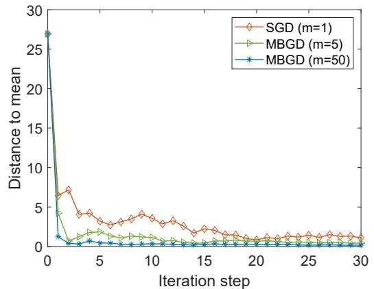
Figure 6.5: An example for demonstrating stochastic and mini-batch gradient descent algorithms. The distribution of X∈R2 is uniform in the square area centered at the origin with a side length as 20. The mean is E[X]=0 . The mean estimation is based on 100 i.i.d. samples.
∣wk−w∗∣ . As a result, when wk is far from w∗ , the relative error is small, and SGD behaves like gradient descent. In addition, since δk is proportional to ∣E[X]−xk∣ , the mean of δk is proportional to the variance of X .
The simulation results are shown in Figure 6.5. Here, X∈R2 represents a random position in the plane. Its distribution is uniform in the square area centered at the origin and E[X]=0 . The mean estimation is based on 100 i.i.d. samples. Although the initial guess of the mean is far away from the true value, it can be seen that the SGD estimate quickly approaches the neighborhood of the origin. When the estimate is close to the origin, the convergence process exhibits certain randomness.
6.4.3 A deterministic formulation of SGD
The formulation of SGD in (6.13) involves random variables. One may often encounter a deterministic formulation of SGD without involving any random variables.
In particular, consider a set of real numbers {xi}i=1n , where xi does not have to be a sample of any random variable. The optimization problem to be solved is to minimize the average:
wminJ(w)=n1i=1∑nf(w,xi),
where f(w,xi) is a parameterized function, and w is the parameter to be optimized. The gradient descent algorithm for solving this problem is
Suppose that the set {xi}i=1n is large and we can only fetch a single number each time.
In this case, it is favorable to update wk in an incremental manner:
wk+1=wk−αk∇wf(wk,xk).(6.16)
It must be noted that xk here is the number fetched at time step k instead of the k th element in the set {xi}i=1n .
The algorithm in (6.16) is very similar to SGD, but its problem formulation is subtly different because it does not involve any random variables or expected values. Then, many questions arise. For example, is this algorithm SGD? How should we use the finite set of numbers {xi}i=1n ? Should we sort these numbers in a certain order and then use them one by one, or should we randomly sample a number from the set?
A quick answer to the above questions is that, although no random variables are involved in the above formulation, we can convert the deterministic formulation to the stochastic formulation by introducing a random variable. In particular, let X be a random variable defined on the set {xi}i=1n . Suppose that its probability distribution is uniform such that p(X=xi)=1/n . Then, the deterministic optimization problem becomes a stochastic one:
wminJ(w)=n1i=1∑nf(w,xi)=E[f(w,X)].
The last equality in the above equation is strict instead of approximate. Therefore, the algorithm in (6.16) is SGD, and the estimate converges if xk is uniformly and independently sampled from {xi}i=1n . Note that xk may repeatedly take the same number in {xi}i=1n since it is sampled randomly.
6.4.4 BGD, SGD, and mini-batch GD
While SGD uses a single sample in every iteration, we next introduce mini-batch gradient descent (MBGD), which uses a few more samples in every iteration. When all samples are used in every iteration, the algorithm is called batch gradient descent (BGD).
In particular, suppose that we would like to find the optimal solution that can minimize J(w)=E[f(w,X)] given a set of random samples {xi}i=1n of X . The BGD, SGD, and MBGD algorithms for solving this problem are, respectively,
wk+1=wk−αkn1i=1∑n∇wf(wk,xi),(B G D)
wk+1=wk−αkm1j∈Ik∑∇wf(wk,xj),(M B G D)
wk+1=wk−αk∇wf(wk,xk).(S G D)
In the BGD algorithm, all the samples are used in every iteration. When n is large, (1/n)∑i=1n∇wf(wk,xi) is close to the true gradient E[∇wf(wk,X)] . In the MBGD al-
gorithm, Ik is a subset of {1,…,n} obtained at time k . The size of the set is ∣Ik∣=m . The samples in Ik are also assumed to be i.i.d. In the SGD algorithm, xk is randomly sampled from {xi}i=1n at time k .
MBGD can be viewed as an intermediate version between SGD and BGD. Compared to SGD, MBGD has less randomness because it uses more samples instead of just one as in SGD. Compared to BGD, MBGD does not require using all the samples in every iteration, making it more flexible. If m=1 , then MBGD becomes SGD. However, if m=n , MBGD may not become SGD. This is because MBGD uses n randomly fetched samples, whereas BGD uses all n numbers. These n randomly fetched samples may contain the same number multiple times and hence may not cover all n numbers in {xi}i=1n .
The convergence speed of MBGD is faster than that of SGD in general. This is because SGD uses ∇wf(wk,xk) to approximate the true gradient, whereas MBGD uses (1/m)∑j∈Ik∇wf(wk,xj) , which is closer to the true gradient because the randomness is averaged out. The convergence of the MBGD algorithm can be proven similarly to the SGD case.
A good example for demonstrating the above analysis is the mean estimation problem. In particular, given some numbers {xi}i=1n , our goal is to calculate the mean xˉ=∑i=1nxi/n . This problem can be equivalently stated as the following optimization problem:
wminJ(w)=2n1i=1∑n∥w−xi∥2,
whose optimal solution is w∗=xˉ . The three algorithms for solving this problem are, respectively,
where xˉk(m)=∑j∈Ikxj/m . Furthermore, if αk=1/k , the above equations can be solved
as follows:
wk+1=k1j=1∑kxˉ=xˉ,(BGD)
wk+1=k1j=1∑kxˉj(m),(M B G D)
wk+1=k1j=1∑kxj.(S G D)
The derivation of the above equations is similar to that of (6.3) and is omitted here. It can be seen that the estimate given by BGD at each step is exactly the optimal solution w∗=xˉ . MBGD converges to the mean faster than SGD because xˉk(m) is already an average.
A simulation example is given in Figure 6.5 to demonstrate the convergence of MBGD. Let αk=1/k . It is shown that all MBGD algorithms with different mini-batch sizes can converge to the mean. The case with m=50 converges the fastest, while SGD with m=1 is the slowest. This is consistent with the above analysis. Nevertheless, the convergence rate of SGD is still fast, especially when wk is far from w∗ .
6.4.5 Convergence of SGD
The rigorous proof of the convergence of SGD is given as follows.
Theorem 6.4 (Convergence of SGD). For the SGD algorithm in (6.13), if the following conditions are satisfied, then wk converges to the root of ∇wE[f(w,X)]=0 almost surely.
(a) 0<c1≤∇w2f(w,X)≤c2 ; (b) ∑k=1∞ak=∞ and ∑k=1∞ak2<∞ ; (c) {xk}k=1∞ are i.i.d.
The three conditions in Theorem 6.4 are discussed below.
⋄ Condition (a) is about the convexity of f . It requires the curvature of f to be bounded from above and below. Here, w is a scalar, and so is ∇w2f(w,X) . This condition can be generalized to the vector case. When w is a vector, ∇w2f(w,X) is the well-known Hessian matrix. ⋄ Condition (b) is similar to that of the RM algorithm. In fact, the SGD algorithm is a special RM algorithm (as shown in the proof in Box 6.1). In practice, ak is often selected as a sufficiently small constant. Although condition (b) is not satisfied in this case, the algorithm can still converge in a certain sense [24, Section 1.5]. Condition (c) is a common requirement.
Box 6.1: Proof of Theorem 6.4
We next show that the SGD algorithm is a special RM algorithm. Then, the convergence of SGD naturally follows from the RM theorem.
The problem to be solved by SGD is to minimize J(w)=E[f(w,X)] . This problem can be converted to a root-finding problem. That is, finding the root of ∇wJ(w)=E[∇wf(w,X)]=0 . Let
g(w)=∇wJ(w)=E[∇wf(w,X)].
Then, SGD aims to find the root of g(w)=0 . This is exactly the problem solved by the RM algorithm. The quantity that we can measure is g~=∇wf(w,x) , where x is a sample of X . Note that g~ can be rewritten as
which is the same as the SGD algorithm in (6.13). As a result, the SGD algorithm is a special RM algorithm. We next show that the three conditions in Theorem 6.1 are satisfied. Then, the convergence of SGD naturally follows from Theorem 6.1.
Since ∇wg(w)=∇wE[∇wf(w,X)]=E[∇w2f(w,X)] , it follows from c1≤∇w2f(w,X)≤c2 that c1≤∇wg(w)≤c2 . Thus, the first condition in Theorem 6.1 is satisfied. The second condition in Theorem 6.1 is the same as the second condition in this theorem. ⋄ The third condition in Theorem 6.1 requires E[ηk∣Hk]=0 and E[ηk2∣Hk]<∞ . Since {xk} is i.i.d., we have Exk[∇wf(w,xk)]=E[∇wf(w,X)] for all k . Therefore,
E[ηk∣Hk]=E[∇wf(wk,xk)−E[∇wf(wk,X)]∣Hk].
Since Hk={wk,wk−1,…} and xk is independent of Hk , the first term on the right-hand side becomes E[∇wf(wk,xk)∣Hk]=Exk[∇wf(wk,xk)] . The second term becomes E[E[∇wf(wk,X)]∣Hk]=E[∇wf(wk,X)] because E[∇wf(wk,X)] is
a function of wk . Therefore,
E[ηk∣Hk]=Exk[∇wf(wk,xk)]−E[∇wf(wk,X)]=0.
Similarly, it can be proven that E[ηk2∣Hk]<∞ if ∣∇wf(w,x)∣<∞ for all w given any x .
Since the three conditions in Theorem 6.1 are satisfied, the convergence of the SGD algorithm follows.