5.1 Motivating example: Mean estimation

We next introduce the mean estimation problem to demonstrate how to learn from data rather than a model. We will see that mean estimation can be achieved based on Monte Carlo methods, which refer to a broad class of techniques that use stochastic samples to solve estimation problems. The reader may wonder why we care about the mean estimation problem. It is simply because state and action values are both defined as the means of returns. Estimating a state or action value is actually a mean estimation problem.

Consider a random variable $X$ that can take values from a finite set of real numbers denoted as $\mathcal{X}$ . Suppose that our task is to calculate the mean or expected value of $X$ : $\mathbb{E}[X]$ . Two approaches can be used to calculate $\mathbb{E}[X]$ .

$\diamond$ The first approach is model-based. Here, the model refers to the probability distribution of $X$ . If the model is known, then the mean can be directly calculated based on the definition of the expected value:

In this book, we use the terms expected value, mean, and average interchangeably.

$\diamond$ The second approach is model-free. When the probability distribution (i.e., the model) of $X$ is unknown, suppose that we have some samples $\{x_{1}, x_{2}, \ldots, x_{n}\}$ of $X$ . Then, the mean can be approximated as

When $n$ is small, this approximation may not be accurate. However, as $n$ increases, the approximation becomes increasingly accurate. When $n \to \infty$ , we have $\bar{x} \rightarrow \mathbb{E}[X]$ .

This is guaranteed by the law of large numbers: the average of a large number of samples is close to the expected value. The law of large numbers is introduced in Box 5.1.

The following example illustrates the two approaches described above. Consider a coin flipping game. Let random variable $X$ denote which side is showing when the coin lands. $X$ has two possible values: $X = 1$ when the head is showing, and $X = -1$ when the tail is showing. Suppose that the true probability distribution (i.e., the model) of $X$ is

If the probability distribution is known in advance, we can directly calculate the mean as

If the probability distribution is unknown, then we can flip the coin many times and record the sampling results $\{x_{i}\}_{i = 1}^{n}$ . By calculating the average of the samples, we can obtain an estimate of the mean. As shown in Figure 5.2, the estimated mean becomes increasingly accurate as the number of samples increases.

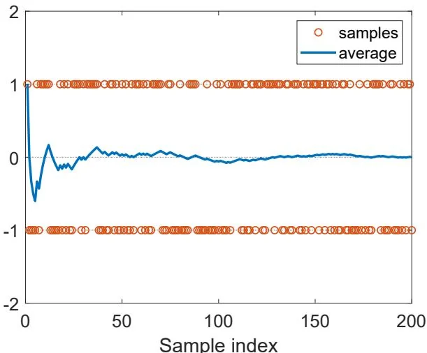
Figure 5.2: An example for demonstrating the law of large numbers. Here, the samples are drawn from $\{+1, -1\}$ following a uniform distribution. The average of the samples gradually converges to zero, which is the true expected value, as the number of samples increases.

It is worth mentioning that the samples used for mean estimation must be independent and identically distributed (i.i.d. or iid). Otherwise, if the sampling values correlate, it may be impossible to correctly estimate the expected value. An extreme case is that all the sampling values are the same as the first one, whatever the first one is. In this case, the average of the samples is always equal to the first sample, no matter how many samples we use.

Box 5.1: Law of large numbers

For a random variable $X$ , suppose that $\{x_{i}\}_{i = 1}^{n}$ are some i.i.d. samples. Let $\bar{x} = \frac{1}{n}\sum_{i = 1}^{n}x_{i}$ be the average of the samples. Then,

The above two equations indicate that $\bar{x}$ is an unbiased estimate of $\mathbb{E}[X]$ , and its variance decreases to zero as $n$ increases to infinity.

The proof is given below.

First, $\mathbb{E}[\bar{x}] = \mathbb{E}\big[\sum_{i = 1}^{n}x_{i} / n\big] = \sum_{i = 1}^{n}\mathbb{E}[x_{i}] / n = \mathbb{E}[X]$ , where the last equability is due to the fact that the samples are identically distributed (that is, $\mathbb{E}[x_i] = \mathbb{E}[X]$ ).

Second, $\operatorname{var}(\bar{x}) = \operatorname{var}\left[\sum_{i=1}^{n} x_i / n\right] = \sum_{i=1}^{n} \operatorname{var}[x_i] / n^2 = (n \cdot \operatorname{var}[X]) / n^2 = \operatorname{var}[X] / n$ , where the second equality is due to the fact that the samples are independent, and the third equability is a result of the samples being identically distributed (that is, $\operatorname{var}[x_i] = \operatorname{var}[X]$ ).