Overview of this Book

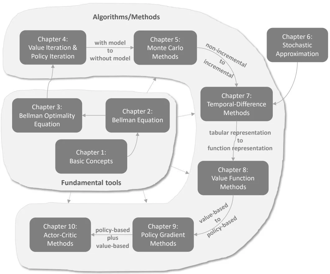
Figure 1: The map of this book.

Before we start the journey, it is important to look at the "map" of the book shown in Figure 1. This book contains ten chapters, which can be classified into two parts: the first part is about basic tools, and the second part is about algorithms. The ten chapters are highly correlated. In general, it is necessary to study the earlier chapters first before the later ones.

Next, please follow me on a quick tour through the ten chapters. Two aspects of each chapter will be covered. The first aspect is the contents introduced in each chapter, and the second aspect is its relationships with the previous and subsequent chapters. A heads up for you to read this overview is as follows. The purpose of this overview is to give you an impression of the contents and structure of this book. It is all right if you encounter many concepts you do not understand. Hopefully, you can make a proper study plan

that is suitable for you after reading this overview.

$\diamond$ Chapter 1 introduces the basic concepts such as states, actions, rewards, returns, and policies, which are widely used in the subsequent chapters. These concepts are first introduced based on a grid world example, where a robot aims to reach a prespecified target. Then, the concepts are introduced in a more formal manner based on the framework of Markov decision processes.

Chapter 2 introduces two key elements. The first is a key concept, and the second is a key tool. The key concept is the state value, which is defined as the expected return that an agent can obtain when starting from a state if it follows a given policy. The greater the state value is, the better the corresponding policy is. Thus, state values can be used to evaluate whether a policy is good or not.

The key tool is the Bellman equation, which can be used to analyze state values. In a nutshell, the Bellman equation describes the relationship between the values of all states. By solving the Bellman equation, we can obtain the state values. Such a process is called policy evaluation, which is a fundamental concept in reinforcement learning. Finally, this chapter introduces the concept of action values.

Chapter 3 also introduces two key elements. The first is a key concept, and the second is a key tool. The key concept is the optimal policy. An optimal policy has the greatest state values compared to other policies. The key tool is the Bellman optimality equation. As its name suggests, the Bellman optimality equation is a special Bellman equation.

Here is a fundamental question: what is the ultimate goal of reinforcement learning? The answer is to obtain optimal policies. The Bellman optimality equation is important because it can be used to obtain optimal policies. We will see that the Bellman optimality equation is elegant and can help us thoroughly understand many fundamental problems.

The first three chapters constitute the first part of this book. This part lays the necessary foundations for the subsequent chapters. Starting in Chapter 4, the book introduces algorithms for learning optimal policies.

Chapter 4 introduces three algorithms: value iteration, policy iteration, and truncated policy iteration. The three algorithms have close relationships with each other. First, the value iteration algorithm is exactly the algorithm introduced in Chapter 3 for solving the Bellman optimality equation. Second, the policy iteration algorithm is an extension of the value iteration algorithm. It is also the foundation for Monte Carlo (MC) algorithms introduced in Chapter 5. Third, the truncated policy iteration algorithm is a unified version that includes the value iteration and policy iteration algorithms as special cases.

The three algorithms share the same structure. That is, every iteration has two steps. One step is to update the value, and the other step is to update the policy. The idea of the interaction between value and policy updates widely exists in reinforcement learning algorithms. This idea is also known as generalized policy iteration. In addition, the algorithms introduced in this chapter are actually dynamic programming algorithms, which require system models. By contrast, all the algorithms introduced in the subsequent chapters do not require models. It is important to well understand the contents of this chapter before proceeding to the subsequent ones.

Starting in Chapter 5, we introduce model-free reinforcement learning algorithms that do not require system models. While this is the first time we introduce model-free algorithms in this book, we must fill a knowledge gap: how to find optimal policies without models? The philosophy is simple. If we do not have a model, we must have some data. If we do not have data, we must have a model. If we have neither, then we can do nothing. The "data" in reinforcement learning refers to the experience samples generated when the agent interacts with the environment.

This chapter introduces three algorithms based on MC estimation that can learn optimal policies from experience samples. The first and simplest algorithm is MC Basic, which can be readily obtained by extending the policy iteration algorithm introduced in Chapter 4. Understanding the MC Basic algorithm is important for grasping the fundamental idea of MC-based reinforcement learning. By extending this algorithm, we further introduce two more complicated but more efficient MC-based algorithms. The fundamental trade-off between exploration and exploitation is also elaborated in this chapter.

Up to this point, the reader may have noticed that the contents of these chapters are highly correlated. For example, if we want to study the MC algorithms (Chapter 5), we must first understand the policy iteration algorithm (Chapter 4). To study the policy iteration algorithm, we must first know the value iteration algorithm (Chapter 4). To comprehend the value iteration algorithm, we first need to understand the Bellman optimality equation (Chapter 3). To understand the Bellman optimality equation, we need to study the Bellman equation (Chapter 2) first. Therefore, it is highly recommended to study the chapters one by one. Otherwise, it may be difficult to understand the contents in the later chapters.

$\diamond$ There is a knowledge gap when we move from Chapter 5 to Chapter 7: the algorithms in Chapter 7 are incremental, but the algorithms in Chapter 5 are non-incremental. Chapter 6 is designed to fill this knowledge gap by introducing the stochastic approximation theory. Stochastic approximation refers to a broad class of stochastic iterative algorithms for solving root-finding or optimization problems. The classic Robbins-Monro and stochastic gradient descent algorithms are special stochastic approximation algorithms. Although this chapter does not introduce any reinforcement

learning algorithms, it is important because it lays the necessary foundations for s-tudying Chapter 7.

Chapter 7 introduces the classic temporal-difference (TD) algorithms. With the preparation in Chapter 6, I believe the reader will not be surprised when seeing the TD algorithms. From a mathematical point of view, TD algorithms can be viewed as stochastic approximation algorithms for solving the Bellman or Bellman optimality equations. Like Monte Carlo learning, TD learning is also model-free, but it has some advantages due to its incremental form. For example, it can learn in an online manner: it can update the value estimate every time an experience sample is received. This chapter introduces quite a few TD algorithms such as Sarsa and Q-learning. The important concepts of on-policy and off-policy are also introduced.
Chapter 8 introduces the value function approximation method. In fact, this chapter continues to introduce TD algorithms, but it uses a different way to represent state/action values. In the preceding chapters, state/action values are represented by tables. The tabular method is straightforward to understand, but it is inefficient for handling large state or action spaces. To solve this problem, we can employ the value function approximation method. The key to understanding this method is to understand the three steps in its optimization formulation. The first step is to select an objective function for defining optimal policies. The second step is to derive the gradient of the objective function. The third step is to apply a gradient-based algorithm to solve the optimization problem. This method is important because it has become the standard technique to represent values. It is also the location in which artificial neural networks are incorporated into reinforcement learning as function approximators. The famous deep Q-learning algorithm is also introduced in this chapter.
Chapter 9 introduces the policy gradient method, which is the foundation of many modern reinforcement learning algorithms. The policy gradient method is policy-based. It is a large step forward in this book because all the methods in the previous chapters are value-based. The basic idea of the policy gradient method is simple: it selects an appropriate scalar metric and then optimizes it via a gradient-ascent algorithm. Chapter 9 has an intimate relationship with Chapter 8 because they both rely on the idea of function approximation. The advantages of the policy gradient method are numerous. For example, it is more efficient for handling large state/action spaces. It has stronger generalization abilities and is more efficient in sample usage.
$\diamond$ Chapter 10 introduces actor-critic methods. From one point of view, actor-critic refers to a structure that incorporates both policy-based and value-based methods. From another point of view, actor-critic methods are not new since they still fall into the scope of the policy gradient method. Specifically, they can be obtained by extending the policy gradient algorithm introduced in Chapter 9. It is necessary for the reader to properly understand the contents in Chapters 8 and 9 before studying Chapter 10.

Chapter 1

Basic Concepts

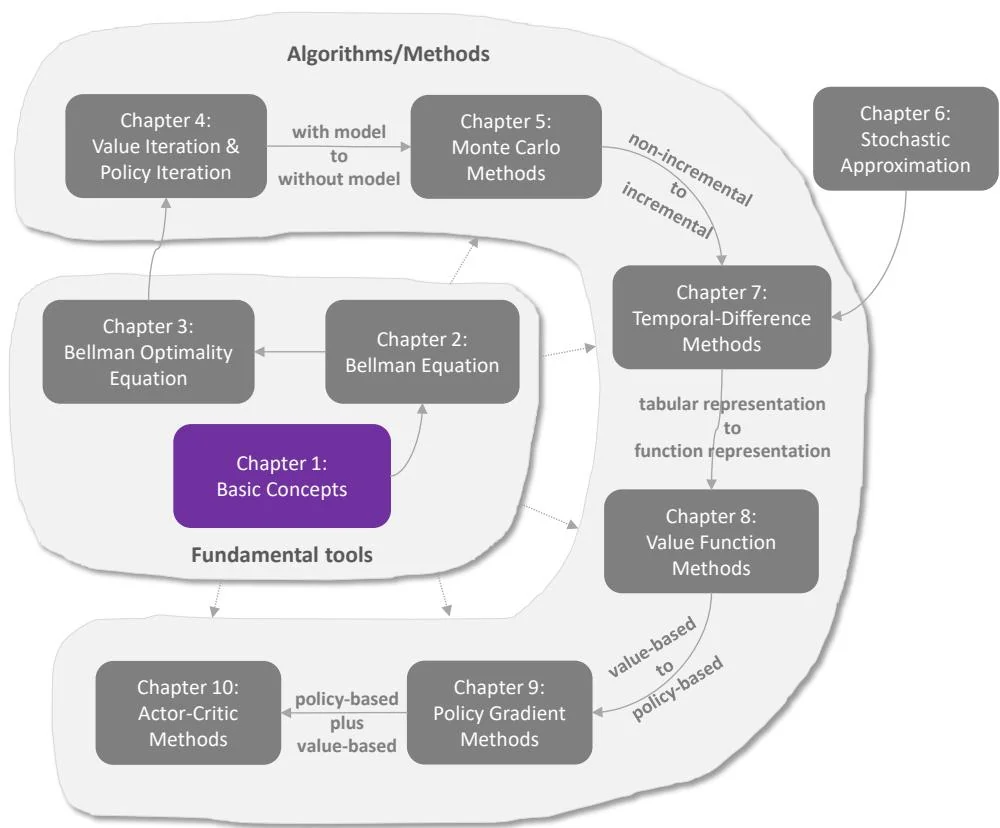
Figure 1.1: Where we are in this book.

This chapter introduces the basic concepts of reinforcement learning. These concepts are important because they will be widely used in this book. We first introduce these concepts using examples and then formalize them in the framework of Markov decision processes.