4.3 Truncated policy iteration

We next introduce a more general algorithm called truncated policy iteration. We will see that the value iteration and policy iteration algorithms are two special cases of the truncated policy iteration algorithm.

4.3.1 Comparing value iteration and policy iteration

First of all, we compare the value iteration and policy iteration algorithms by listing their steps as follows.

$\diamond$ Policy iteration: Select an arbitrary initial policy $\pi_0$ . In the $k$ th iteration, do the following two steps.

• Step 1: Policy evaluation (PE). Given $\pi_k$ , solve $v_{\pi_k}$ from

• Step 2: Policy improvement (PI). Given $v_{\pi_k}$ , solve $\pi_{k+1}$ from

$\diamond$ Value iteration: Select an arbitrary initial value $v_0$ . In the $k$ th iteration, do the following two steps.

• Step 1: Policy update (PU). Given $v_{k}$ , solve $\pi_{k + 1}$ from

• Step 2: Value update (VU). Given $\pi_{k+1}$ , solve $v_{k+1}$ from

The above steps of the two algorithms can be illustrated as

Policy iteration: $\pi_0 \xrightarrow{PE} v_{\pi_0} \xrightarrow{PI} \pi_1 \xrightarrow{PE} v_{\pi_1} \xrightarrow{PI} \pi_2 \xrightarrow{PE} v_{\pi_2} \xrightarrow{PI} \dots$

Value iteration: $v_{0} \xrightarrow{PU} \pi_{1}^{\prime} \xrightarrow{VU} v_{1} \xrightarrow{PU} \pi_{2}^{\prime} \xrightarrow{VU} v_{2} \xrightarrow{PU} \ldots$

It can be seen that the procedures of the two algorithms are very similar.

We examine their value steps more closely to see the difference between the two algorithms. In particular, let both algorithms start from the same initial condition: $v_{0} = v_{\pi_{0}}$ . The procedures of the two algorithms are listed in Table 4.6. In the first three steps, the two algorithms generate the same results since $v_{0} = v_{\pi_{0}}$ . They become

Table 4.6: A comparison between the implementation steps of policy iteration and value iteration.

different in the fourth step. During the fourth step, the value iteration algorithm executes $v_{1} = r_{\pi_{1}} + \gamma P_{\pi_{1}}v_{0}$ , which is a one-step calculation, whereas the policy iteration algorithm solves $v_{\pi_1} = r_{\pi_1} + \gamma P_{\pi_1}v_{\pi_1}$ , which requires an infinite number of iterations. If we explicitly write out the iterative process for solving $v_{\pi_1} = r_{\pi_1} + \gamma P_{\pi_1}v_{\pi_1}$ in the fourth step, everything becomes clear. By letting $v_{\pi_1}^{(0)} = v_0$ , we have

The following observations can be obtained from the above process.

If the iteration is run only once, then $v_{\pi_1}^{(1)}$ is actually $v_{1}$ , as calculated in the value iteration algorithm.
If the iteration is run an infinite number of times, then $v_{\pi_1}^{(\infty)}$ is actually $v_{\pi_1}$ , as calculated in the policy iteration algorithm.
If the iteration is run a finite number of times (denoted as $j_{\mathrm{truncated}}$ ), then such an algorithm is called truncated policy iteration. It is called truncated because the remaining iterations from $j_{\mathrm{truncated}}$ to $\infty$ are truncated.

As a result, the value iteration and policy iteration algorithms can be viewed as two extreme cases of the truncated policy iteration algorithm: value iteration terminates

Algorithm 4.3: Truncated policy iteration algorithm
Initialization: The probability models $p(r|s,a)$ and $p(s'|s,a)$ for all $(s,a)$ are known. Initial guess $\pi_0$ .
Goal: Search for the optimal state value and an optimal policy.
While $v_k$ has not converged, for the $k$ th iteration, do
Policy evaluation:
Initialization: select the initial guess as $v_k^{(0)} = v_{k-1}$ . The maximum number of iterations is set as $j_{\text{truncated}}$ .
While $j < j_{\text{truncated}}$ , do
For every state $s \in S$ , do
$v_k^{(j+1)}(s) = \sum_a \pi_k(a|s) \left[ \sum_r p(r|s,a)r + \gamma \sum_{s'} p(s'|s,a)v_k^{(j)}(s') \right]$
Set $v_k = v_k^{(j_{\text{truncated}})}$
Policy improvement:
For every state $s \in S$ , do
For every action $a \in \mathcal{A}(s)$ , do
$q_k(s,a) = \sum_r p(r|s,a)r + \gamma \sum_{s'} p(s'|s,a)v_k(s')$ $a_k^*(s) = \arg \max_a q_k(s,a)$ $\pi_{k+1}(a|s) = 1$ if $a = a_k^*$ , and $\pi_{k+1}(a|s) = 0$ otherwise

at $j_{\mathrm{truncate}} = 1$ , and policy iteration terminates at $j_{\mathrm{truncate}} = \infty$ . It should be noted that, although the above comparison is illustrative, it is based on the condition that $v_{\pi_1}^{(0)} = v_0 = v_{\pi_0}$ . The two algorithms cannot be directly compared without this condition.

4.3.2 Truncated policy iteration algorithm

In a nutshell, the truncated policy iteration algorithm is the same as the policy iteration algorithm except that it merely runs a finite number of iterations in the policy evaluation step. Its implementation details are summarized in Algorithm 4.3. It is notable that $v_{k}$ and $v_{k}^{(j)}$ in the algorithm are not state values. Instead, they are approximations of the true state values because only a finite number of iterations are executed in the policy evaluation step.

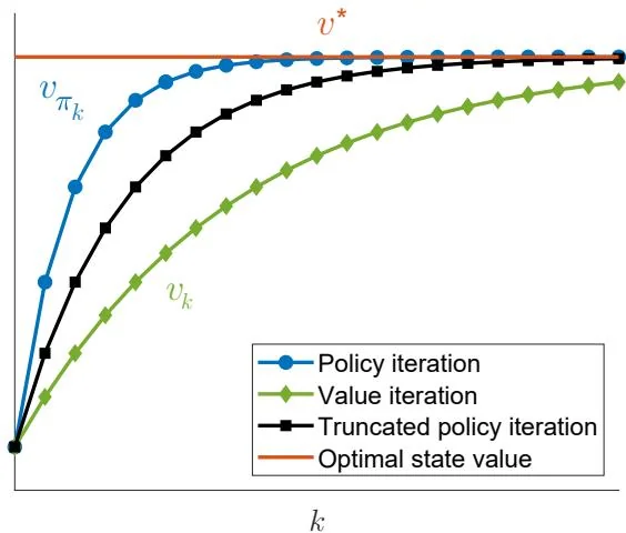
If $v_{k}$ does not equal $v_{\pi_k}$ , will the algorithm still be able to find optimal policies? The answer is yes. Intuitively, truncated policy iteration is in between value iteration and policy iteration. On the one hand, it converges faster than the value iteration algorithm because it computes more than one iteration during the policy evaluation step. On the other hand, it converges slower than the policy iteration algorithm because it only computes a finite number of iterations. This intuition is illustrated in Figure 4.5. Such intuition is also supported by the following analysis.

Proposition 4.1 (Value improvement). Consider the iterative algorithm in the policy

Figure 4.5: An illustration of the relationships between the value iteration, policy iteration, and truncated policy iteration algorithms.

evaluation step:

If the initial guess is selected as $v_{\pi_k}^{(0)} = v_{\pi_{k - 1}}$ , it holds that

for $j = 0,1,2,\ldots$

Box 4.3: Proof of Proposition 4.1

First, since $v_{\pi_k}^{(j)} = r_{\pi_k} + \gamma P_{\pi_k}v_{\pi_k}^{(j - 1)}$ and $v_{\pi_k}^{(j + 1)} = r_{\pi_k} + \gamma P_{\pi_k}v_{\pi_k}^{(j)}$ , we have

Second, since $v_{\pi_k}^{(0)} = v_{\pi_{k - 1}}$ , we have

where the inequality is due to $\pi_k = \arg \max_{\pi}(r_\pi + \gamma P_\pi v_{\pi_{k-1}})$ . Substituting $v_{\pi_k}^{(1)} \geq v_{\pi_k}^{(0)}$ into (4.5) yields $v_{\pi_k}^{(j+1)} \geq v_{\pi_k}^{(j)}$ .

Notably, Proposition 4.1 requires the assumption that $v_{\pi_k}^{(0)} = v_{\pi_{k-1}}$ . However, $v_{\pi_{k-1}}$ is unavailable in practice, and only $v_{k-1}$ is available. Nevertheless, Proposition 4.1 still sheds light on the convergence of the truncated policy iteration algorithm. A more in-depth discussion of this topic can be found in [2, Section 6.5].

Up to now, the advantages of truncated policy iteration are clear. Compared to the

policy iteration algorithm, the truncated one merely requires a finite number of iterations in the policy evaluation step and hence is more computationally efficient. Compared to value iteration, the truncated policy iteration algorithm can speed up its convergence rate by running for a few more iterations in the policy evaluation step.