13.3 Scan and Circuit Design

Having explored one possible parallel algorithm for Scan, it may now be clear that there are many different ways to implement parallel Scan algorithms. In reasoning about other possible implementations, we can take advantage of design methodologies for integer addition hardware that performs a similar function: Instead of propagating an arbitrary binary associative operator $\oplus$ across an array, culminating in the output from a reduction, hardware adders propagate partial addition results, culminating in the carry bit to be propagated for multiprecision arithmetic.

Hardware designers use directed acyclic, oriented graphs to represent different implementations of Scan "circuits." These diagrams compactly express both the data flow and the parallelism. A diagram of the serial implementation of Listing 13.1 is given in Figure 13.6. The steps proceed downward as time advances; the vertical lines denote wires where the signal is propagated. Nodes of in-degree 2 ("operation nodes") apply the operator $\oplus$ to their inputs.

Note that the circuit diagrams show inclusive scans, not exclusive ones. For circuit diagrams, the difference is minor; to turn the inclusive scan in Figure 13.6 into an exclusive scan, a 0 is wired into the first output and the sum is wired into the output, as shown in Figure 13.7. Note that both inclusive and exclusive scans generate the reduction of the input array as output, a characteristic that we will exploit in building efficient scan algorithms. (For purposes of clarity, all circuit diagrams other than Figure 13.7 will depict inclusive scans.)

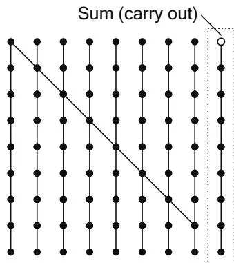
Figure 13.6 Serial scan.

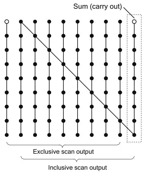
Figure 13.7 Serial scan (inclusive and exclusive).

The Scan algorithm described by Blelloch corresponds to a circuit design known as Brent-Kung, a recursive decomposition in which every second output is fed into a Brent-Kung circuit of half the width. Figure 13.8 illustrates a Brent-Kung circuit operating on our example length of 8, along with Blelloch's upsweep and downsweep phases. Nodes that broadcast their output to multiple nodes in the next stage are known as fans. Brent-Kung circuits are notable for having a constant fan-out of 2.

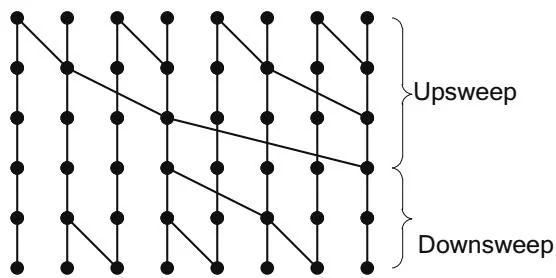
Figure 13.8 Brent-Kung circuit.

The structure of a Brent-Kung circuit becomes clearer on larger circuits; see, for example, the circuit that processes 16 inputs in Figure 13.9. Figure 13.9 also highlights the spine of the circuit, the longest subgraph that generates the last element of the scan output.

The depth of the Brent-Kung circuit grows logarithmically in the number of inputs, illustrating its greater efficiency than (for example) the serial algorithm. But because each stage in the recursive decomposition increases the depth by 2, the Brent-Kung circuit is not of minimum depth. Sklansky described a method to build circuits of minimum depth by recursively decomposing them as shown in Figure 13.10.

Two $(N / 2)$ -input circuits are run in parallel, and the output of the spine of the left circuit is added to each element of the right circuit. For our 16-element example, the left-hand subgraph of the recursion is highlighted in Figure 13.10.

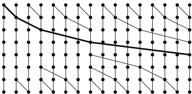
Figure 13.9 Brent-Kung circuit (16 inputs).

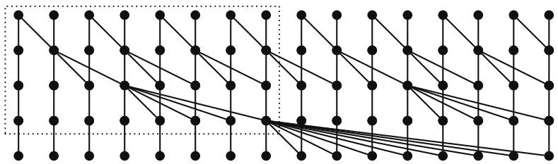
Figure 13.10 Sklansky (minimum-depth) circuit.

Another minimum-depth scan circuit, known as Kogge-Stone, has a constant fan-out of 2, which is a desirable characteristic for hardware implementation, but, as you can see in Figure 13.11, it has many operation nodes; software implementations analogous to Kogge-Stone are work-inefficient.

Any scan circuit can be constructed from a combination of scans (which perform the parallel prefix computation and generate the sum of the input array as output) and fans (which add an input to each of their remaining outputs). The minimum-depth circuit in Figure 13.10 makes heavy use of fans in its recursive definition.

For an optimized CUDA implementation, a key insight is that a fan doesn't need to take its input from a Scan per se; any reduction will do. And from Chapter 12, we have a highly optimized reduction algorithm.

If, for example, we split the input array into subarrays of length $b$ and compute the sum of each subarray using our optimized reduction routine, we end up with an array of $\left\lceil \frac{N}{b} \right\rceil$ reduction values. If we then perform an exclusive scan on

that array, it becomes an array of fan inputs (seeds) for scans of each subarray. The number of values that can be efficiently scanned in one pass over global memory is limited by CUDA's thread block and shared memory size, so for larger inputs, the approach must be applied recursively.

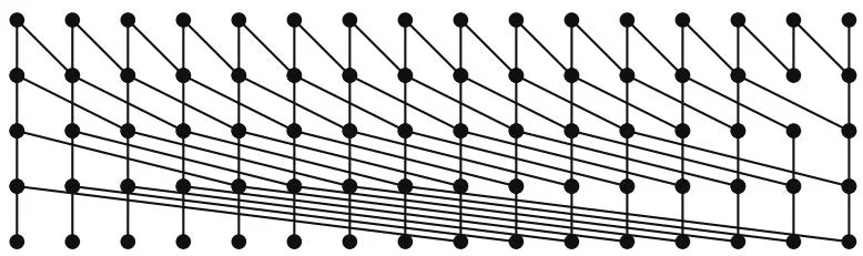
Figure 13.11Kogge-Stone circuit.